Updating BISG Proxies: How 2020 Census Data Impacts Fair Lending Risk
- Richard Pace, PhD

- Aug 8, 2023
- 28 min read
Updated: Apr 16
A primary tool for identifying disparate impact, the BISG Model itself ironically appears to suffer from its own growing disparate impact - particularly for Black Americans.

For the last twelve years, many bank regulatory and enforcement agencies, and scores of non-mortgage consumer lenders, have employed the Bayesian Improved Surname Geocoding ("BISG") race/ethnicity proxy model to analyze consumer lending outcomes for evidence of potential discrimination. Such proxy usage has expanded even further in recent years as these same lenders and fintechs use the model to help purge "algorithmic bias" from their increasingly-complex consumer loan decisioning algorithms,[1] and digital advertisers incorporate it into sophisticated tools to reduce the disparate impact of their housing, employment, and credit ad delivery systems powered by alternative data and machine learning technology.[2]
In 2021, I published the first comprehensive analysis of the BISG proxy model for fair lending compliance risk management purposes - focusing on its inherent predictive accuracy at the aggregate and individual borrower levels, and evaluating its ability to estimate accurately disparate treatment and disparate impact pricing disparities for Black, Hispanic, and Asian & Pacific Islander ("API") groups (relative to Whites). While a complete summary of my prior study's findings is outside the scope of this post, I note below a few of the salient observations based on the proxy model's then-current usage of 2010 U.S. Census geographical and surname demographic data (the "2010 BISG Model"):
When used to estimate the aggregate race/ethnicity composition of a borrower sample, the 2010 BISG Model produces unbiased and accurate estimates so long as the characteristics of the consumer sample are statistically aligned with the characteristics of the U.S. Census data serving as inputs to the proxy model. However, should the sample deviate from these characteristics - for example, by being concentrated in certain states, in higher-income consumer segments, or simply due to demographic drifts over time, then aggregate-level proxy inaccuracies emerge with magnitudes that vary based on the nature and severity of the specific deviations.
When used to classify the specific race/ethnicity of 2010 sample borrowers, the 2010 BISG Model inaccurately predicts the race of Black adults 42 - 73% of the time (depending on which individual-level classification rule is employed) – a significantly larger error rate than for Whites (7 - 25%). Hispanics (22 - 52%) and APIs (34 - 58%) also exhibit relatively high individual-level prediction errors.
Drilling down into the individual-level prediction errors for Blacks, I noted that the 2010 BISG Model fails to include higher-income Blacks residing in racially-diverse neighborhoods in the "Predicted Black" group, while inaccurately including lower-income Whites residing in high-minority neighborhoods. Accordingly, the socioeconomic characteristics of 2010 sample members predicted to be Black are biased from their true values – having much lower average median incomes and being much more concentrated in high-minority neighborhoods that Actual Blacks.
Because of these inaccurate and biased race/ethnicity predictions, I found that:
Under disparate treatment scenarios – whereby lender discrimination is based on actual race/ethnicity – all 2010 BISG Classification approaches cause an underestimation of true minority price disparities by 9 - 34%. Alternatively, the BISG Continuous estimation approach[3] produced unbiased minority disparity estimates - but only when the characteristics of the borrower sample were statistically aligned with the characteristics of the U.S. Census data serving as inputs to the 2010 BISG Model. If such sample data alignment is not present - for example, because of regional or local samples, samples skewed toward higher income individuals, or due to aging of the BISG Model's Census data inputs - then these disparity estimates will also be biased.
Under a disparate impact scenario where discretionary pricing is correlated with borrower income levels, both the BISG Classification and Continuous estimation approaches produced biased minority price disparity estimates. Under the BISG Classification approaches, these biases ranged between -10% and +80% while, under the BISG Continuous approach, price disparity estimates were inflated by 80-100% for Hispanic and Black groups (relative to Whites).
Overall, this evidence strongly indicates that the BISG Model, a primary tool of federal and state bank regulators and enforcement agencies to root out illegal disparate impact, ironically appears to suffer from its own disparate impact - in many cases significantly mis-identifying U.S. minorities, underestimating disparate treatment disparities, and overestimating disparate impact disparities - particularly for Black adults.
In May 2023, a year and a half after my 2021 Study was released, the U.S. Census Bureau finally released updated geo-demographic data from the 2020 U.S. Census that improves the alignment of the BISG Model with current U.S. population demographics. Given this update, the following important questions naturally arise from a fair lending compliance risk management perspective:
How does this update impact the inherent accuracy of the 2020 BISG Model relative to the 2010 BISG Model (i.e., on concurrent borrower samples)?
How will the updated 2020 BISG Model's race/ethnicity probabilities impact the magnitude of potential fair lending disparity estimate biases on current borrower samples relative to those identified in my 2021 study (which focused on 2010 borrower samples)?
For current borrower samples, what are the potential consequences of not adopting the 2020 BISG Model - that is, continuing to use the 2010 model version?
In this post, I address these questions - and revisit the model's apparent disparate impact - using the same analytical framework as I used in my 2021 study, but with an updated 2020 BISG Model (assuming no changes to the CFPB's BISG proxy methodology) and a current borrower sample. While prior reading of my 2021 BISG study is not absolutely necessary to access the results below, it does provide helpful context as well as much greater insights as to my data, my methodologies, and the underlying intuition behind the results obtained. With that qualification...
Let's dive in.
1. Creating the 2020 BISG Model
Consistent with the 2010 U.S. Census geo-demographic dataset described in the CFPB's published methodology document and in their associated GitHub materials, my 2020 BISG Model uses the updated Census Block Group ("CBG")-level P11 Table (Hispanic or Latino, and Not Hispanic or Latino by Race for the Population 18 Years and Over) from the 2020 U.S. Census Demographics and Housing Characteristics ("DHC") File.[4] This is the only change I make to create the 2020 BISG Model.
Now, before I dive into the updated proxy-based analyses and results associated with the 2020 BISG Model, I believe it's important and helpful to first establish the broader context for these downstream results through an overview of U.S. geo-demographic changes between 2010 and 2020.[5]
2. 2010-2020 U.S. Census Geo-Demographic Changes
2.1. National-Level Demographic Trends
Starting at the highest geographic level, Figure 1 shows that the U.S. adult population - as a whole - has become more racially and ethnically diverse over the last decade with: (1) population shares of Black and Hispanic groups up 0.1 and 2.6 percentage points, respectively, (2) a significant drop of 5.5 percentage points in White representation, and (3) increases in API and multiracial population shares by 1.2 and 1.3 percentage points, respectively.

I note that the U.S. Census Bureau attributes these demographic changes to the effects of both pure demographic change and the Census Bureau's improvements "in the design of the two separate questions for race data collection and processing".[6]
2.2. State-Level Demographic Trends
In addition to the national-level demographic trends, it is also useful to see how state-level demographics have changed over the past decade. To that end, let's first look at how demographic diversity has changed within each state.
Between 2010 and 2020, 41 states increased their population share of Black adults. Figure 2 shows the states with the largest gains in Black representation (relative to their total populations) - North Dakota (+2.0%), Nevada (+1.7%), Minnesota (+1.5%), Georgia (+1.3%), and Delaware (+1.2%). On the opposite end, the District of Columbia (-7.9%), South Carolina (-2.2%), North Carolina (-0.5%), Tennessee (-0.4%), and California (-0.3%) lost the most Black representation.

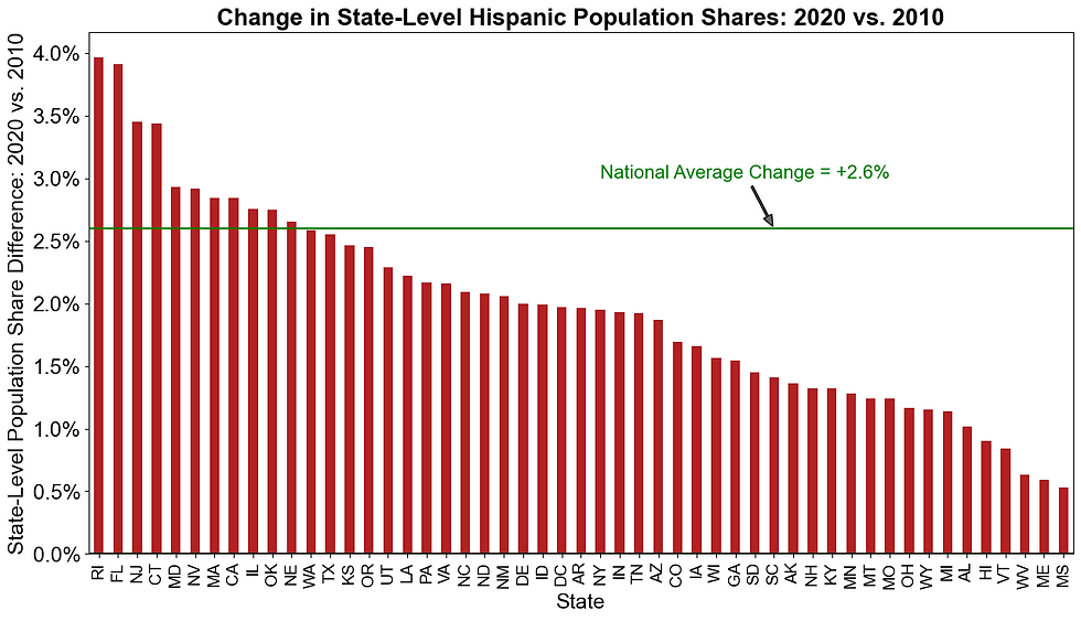
Between 2010 and 2020, all 50 states and the District of Columbia increased their population share of Hispanic adults. Figure 3 shows the biggest gainers in Hispanic representation (relative to their total populations) were Rhode Island (+4.0%), Florida (+3.9%), New Jersey (+3.5%), Connecticut (+3.4%), and Maryland (+2.9%). On the opposite end, Mississippi (+0.5%), Maine (+0.6%), West Virginia (+0.6%), Vermont (+0.8%), and Hawaii (+0.9%) gained the least Hispanic representation.
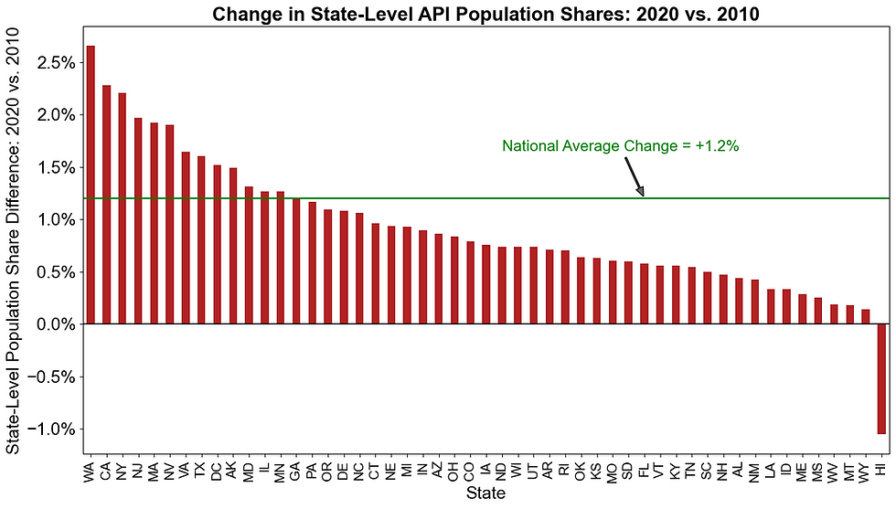
Finally, between 2010 and 2020, 49 states and the District of Columbia increased their population share of API adults. Figure 4 shows the biggest gainers in API representation were Washington (+2.7%), California (+2.3%), New York (+2.2%), New Jersey (+2.0%), and Massachusetts (+1.9%). On the opposite end, Hawaii (-1.1%) lost API representation while Wyoming (+0.1%), Montana (+0.2%), West Virginia (+0.2%), and Mississippi (+0.2%) gained the least.
Now, let's flip our perspective and - instead of looking at demographic changes within states - let's look at each race/ethnicity group's migration across states over the ten-year period between 2010 and 2020. Figure 5 below shows these migration levels for U.S. Black adults. Keep in mind that - when viewing the data from this perspective - one state's gain must be another state's loss so the sum of these state-level changes will necessarily equal zero.[7]

Here we can see that Texas (+0.9%), Georgia (+0.5%), Florida (+0.3%), Minnesota (+0.2%), and Nevada (+0.2%) had the largest Black "in-migration" rates between 2010 and 2020, while California (-0.4%), New York (-0.4%), Illinois (-0.4%), Michigan (-0.3%), and South Carolina (-0.2%) had the largest "out-migration" rates.
Figure 6 below shows these migration levels for U.S. Hispanic adults. Here we can see that Florida (+0.6%), Pennsylvania (+0.2%), Washington (+0.2%), North Carolina (+0.2%), and Massachusetts (+0.2%) had the largest Hispanic "in-migration" rates between 2010 and 2020, while California (-2.2%), New York (-0.6%), New Mexico (-0.3%), Illinois (-0.2%), and Texas (-0.2%) had the largest "out-migration" rates.

Finally, Figure 7 below shows these migration levels for U.S. API adults. Here we can see that Texas (+1.3%), Washington (+0.5%), North Carolina (+0.3%), Georgia (+0.3%), and Massachusetts (+0.2%) had the largest "in-migration" rates of U.S. API adults between 2010 and 2020, while California (-2.5%), Hawaii (-1.1%), Illinois (-0.2%), New Jersey (-0.1%), and Maryland (-0.1%) had the largest "out-migration" rates.

2.3. Neighborhood-Level Demographic Trends
Figure 8 drills down to the lowest geographic level in my data to examine 2010-2020 demographic trends at the "neighborhood" (i.e., CBG) level - which is the micro-geographic level at which the BISG Model typically operates.[8]
2020 vs. 2010 U.S. Census Geo-Demographic Trends - "Neighborhood" Level:
U.S. Adult Population

According to these neighborhood-level metrics:
On average, U.S. Black adults live in more racially-diverse neighborhoods in 2020 vs. 2010 with a 4.1 percentage point lower average Black CBG population share (i.e., 42.1% vs. 46.2% Black). Additionally, only 16.6% of Black adults lived in highly segregated (i.e., >= 80% Black) CBGs in 2020 vs. 22.6% in 2010 - a 27% reduction, while 61.4% of Black adults lived in CBGs with less than 50% Blacks in 2020 vs. 56.5% in 2010 - an 8% increase.
On average, U.S. Hispanic adults also live in slightly more racially-diverse neighborhoods in 2020 vs. 2010 with a 0.6 percentage point lower average Hispanic CBG population share (i.e., 43.2% vs. 43.8%). Additionally, only 15.1% of Hispanic adults lived in highly segregated (i.e., >= 80% Hispanic) CBGs in 2020 vs. 16.5% in 2010 - an 8% reduction, while 60.0% of Hispanic adults lived in CBGs with less than 50% Hispanics vs. 58.8% in 2010 - a 2% increase.
On average, U.S. API adults slightly decreased their residential neighborhood diversity between 2010 and 2020 with a 1.8 percentage point higher average API CBG population share (i.e., 24.9% vs. 23.2%) - with similar small increases (decreases) in the percentage of API adults living in highly segregated (diverse) CBGs.
With this backdrop of national, state, and neighborhood-level demographic changes over the past decade, let's now turn to their impacts on current BISG proxy-based fair lending analyses.
3. The 2020 Borrower Sample
As I discussed on pp. 11-15 of my 2021 BISG Study, due to the lack of a publicly-available, nationally-representative sample of U.S. individuals with the personally-identifiable information needed to generate BISG race/ethnicity proxy probabilities (i.e., last name and residential address), I created a synthetic dataset of such individuals by randomly-sampling from the 2010 U.S. Census CBGs and the 2010 U.S. Census Surnames (according to their respective population shares) to create 10 million CBG-surname combinations. I then used these 2010-based synthetic borrowers to create a corresponding set of race/ethnicity probabilities using the 2010 BISG Model, and then applied Monte Carlo random sampling techniques to assign an "actual" race/ethnicity to each borrower consistent with these underlying probabilities.[9]
Since the 2021 study's synthetic borrower sample was designed to be reflective of 2010 U.S. population demographics, and given the various geo-demographic changes that have occurred since 2010 (see Section 2), I create for the current analysis a new 2020-based synthetic borrower sample using the same methodology as described above, but with updated race/ethnicity probabilities from the 2020 BISG Model and an updated set of "actual" race/ethnicity assignments consistent with these probabilities.
One of the risks in comparing results from the 2010 and 2020 borrower samples is that certain compositional differences between the two samples could introduce statistical noise into the results - thereby confounding somewhat the conclusions that can be drawn. For example, if I completely re-created the set of 10 million CBG-surname combinations for the 2020 synthetic borrower sample, then it is possible that my 2010 vs. 2020 test result differences may be partially attributable to the differences in the specific set of CBG-surname combinations present in the two samples. Therefore, to minimize this risk, I created the 2020 borrower sample as follows:
I used the same set of 10 million CBG-surname combinations as was used for the 2010 borrower sample.
To update each sample member's BISG probabilities using the 2020 BISG Model, I mapped each sample member's 2010 CBG location into its corresponding 2020 CBG location (due to the evolution of CBG boundaries over the past decade).[10] I then used the 2020 CBG location to: (1) merge on the corresponding geo-demographic data from the 2020 U.S. Census and (2) calculate the 2020 BISG race/ethnicity probabilities.
To assign an "actual" race/ethnicity (now reflective of 2020 geo-demographic patterns), I applied the Monte Carlo random sampling technique to each sample member's set of 2020 BISG probabilities using the same random numbers as were used to create the 2010 "actual" race/ethnicities.
4. 2020 U.S. Census Data: Impact on Aggregate BISG Proxy Prediction Accuracy
As highlighted at the beginning of this post, my 2021 BISG study found that the BISG Model produces unbiased and accurate estimates of a sample's aggregate race/ethnicity composition so long as the characteristics of the sample being proxied are statistically aligned with the characteristics of the U.S. Census data serving as inputs to the proxy model. However, should the sample deviate from these Census data characteristics, then aggregate-level proxy inaccuracies emerge with magnitudes that vary based on the nature and severity of the specific deviations.
This conclusion is unaffected by the 2020 update to the U.S. Census geo-demographic data as illustrated below in Figure 9.
2010 and 2020 BISG Models - Absolute and Relative Aggregate Prediction Errors:
2020 Borrower Sample

The first row of this table ("2010 BISG Model") displays the estimated demographic distribution of my 2020 synthetic borrower sample based on the 2010 BISG Model. The second row shows the same estimated distribution but this time using the 2020 BISG Model. Finally, the third row provides the "actual" demographic distribution of my 2020 borrower sample.
The middle set of rows in Figure 9 compute the absolute and relative prediction errors associated with the 2010 BISG Model, while the last set of rows compute the same for the 2020 BISG Model. Consistent with the original study's finding, the 2020 BISG Model exhibits effectively zero aggregate prediction error since the characteristics of the 2020 synthetic borrower sample - by design - are well aligned to the characteristics of the 2020 BISG Model data inputs.
However, should one continue to use the 2010 BISG Model for current borrower samples (middle set of rows), then the drift in the borrower sample characteristics since 2010 will likely result in relative prediction errors. In my broad-based 2020 sample, these errors ranged from -4.6% for the Black relative error rate (i.e., under-predicting the total number of Black adults in the sample) to +1.7% for Whites.
5. 2020 U.S. Census Data: Impact on Individual-Level
BISG Proxy Prediction Accuracy
In this section, I assess the 2020 BISG Model's impacts on individual-level race/ethnicity prediction accuracy using the two most-common BISG classification rules - the BISG Max rule and the BISG 80% Threshold rule.[11] As a quick summary:
The BISG Max classification rule ("BISG Max rule") predicts an individual's race/ethnicity by selecting the specific group with the highest BISG probability. For example, if an individual has the following BISG probabilities: 68.9% White, 0.2% Black, 0.5% API, 30.2% Hispanic, and 0.2% Other, the BISG Max classification rule would assign this individual a predicted race/ethnicity of White since that racial group has the highest probability.
The BISG 80% Threshold classification rule ("BISG 80% rule") predicts an individual's race/ethnicity by selecting the specific group whose BISG probability is at least 80%. If no category achieves this probability threshold, then the individual's predicted race/ethnicity is "Unknown". In our example above, since no group has a probability value of at least 80%, this individual's race/ethnicity would be designated as "Unknown".
A key difference between these two classification rules is that the BISG Max rule provides predictions for 100% of the borrower sample (i.e., a 100% "coverage rate") but exhibits greater uncertainty in its race/ethnicity predictions since some may be based on BISG probability values as low as 21%. Alternatively, the BISG 80% rule has a much lower coverage rate due to the "Unknowns", but it exhibits less uncertainty in the race/ethnicity predictions it does make since the underlying probabilities on which they are based are very high (>= 80%).
Using the same Individual-Level Accuracy assessment framework as on pp. 25-27 of my 2021 BISG Study, Figures 10 and 11 below show the impact of the 2020 BISG Model on individual-level race/ethnicity prediction accuracy under these rules.
5.1. BISG Max Classification Rule Results
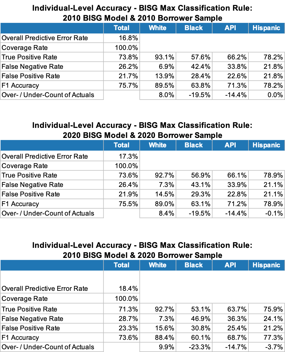
Figure 10 summarizes the BISG Models' individual-level predictive performance under three scenarios. The top table presents the 2010 BISG Model's predictive performance on the 2010 borrower sample (from my 2021 BISG Study). The middle table presents the performance results for the scenario where the lender uses the updated 2020 BISG Model on current borrower samples, and the bottom table pertains to the scenario where the lender continues to use the existing 2010 BISG Model on current borrower samples.
Overall, for typical fair lending race/ethnicity focal points (i.e., Blacks, Hispanics, and APIs), my BISG Max-based analyses of individual-level race/ethnicity prediction indicate that:
The 2020 BISG Model's Overall Predictive Error Rate (i.e., the percentage of actual group members whose race/ethnicity is correctly predicted) on the current borrower sample (the middle table) is 0.5 percentage points higher (a relative increase of 3%) than that of the 2010 BISG Model on the 2010 borrower sample (the top table). This reduction in the 2020 BISG Model's inherent predictive performance is reflective of the general decrease in U.S. race/ethnicity segregation at both the national- and neighborhood levels since 2010 - which, on average, provides less predictive power to the 2020 BISG Model.[12]
For all groups except Hispanic, the 2020 BISG Model (middle table) has higher False Negative Rates (i.e., the percentage of actual group members who are predicted to be members of a different race/ethnicity group) than the 2010 BISG Model (top table). While problematic for all impacted race/ethnicity groups, it is particularly troubling for Black adults as the False Negative Rate was already at a very high level in 2010 (43.1% of Actual Black adults are misclassified using the 2020 BISG Model vs. 42.4% using the 2010 Model) - leading to a significant exclusion of actual Black adults from the fair lending testing associated with their racial group.[13] Hispanic adults, on the other hand, exhibit a modest improvement in their False Negative Rate - decreasing from 21.8% using the 2010 BISG Model to 21.1% for the 2020 BISG Model.[14]
For all groups except Hispanic, the 2020 BISG Model (middle table) also increases the False Positive Rate (i.e., the percentage of predicted group members who are actually members of a different race/ethnicity group) relative to the 2010 BISG Model (top table). For Predicted Black adults, for example, the False Positive Rate increases from 28.4% to 29.3% - indicating that a group of Predicted Blacks in a current borrower sample is actually only 70.7% Black. Not only are the remaining 29.3% of Predicted Black adults actually other races/ethnicities, but over two-thirds of them (68%) are actually White. Hispanic adults, on the other hand, exhibit a modest improvement in their False Positive Rate using the 2020 BISG Model - decreasing from 21.8% to 21.1%.
As measured by the F1 Accuracy metric,[15] overall BISG Max classification accuracy decreased slightly, on average, across the groups by 0.2 percentage points due to the updated 2020 Census geo-demographic data. Across race/ethnicity groups, F1 Accuracy for Black adults decreased the most (0.7 percentage points) while F1 Accuracy for Hispanic adults increased by 0.7 percentage points.
Continuing to use the 2010 BISG Model on current borrower samples (instead of the 2020 BISG Model) for BISG Max-based individual-level race/ethnicity prediction results in a higher overall predictive error rate (+1.1 percentage points, see the bottom table) - with actual Black, Hispanic, and API adults experiencing a +3.9, +3.0, and +2.4 percentage point higher prediction error rate, respectively.
5.2. BISG 80% Classification Rule Results
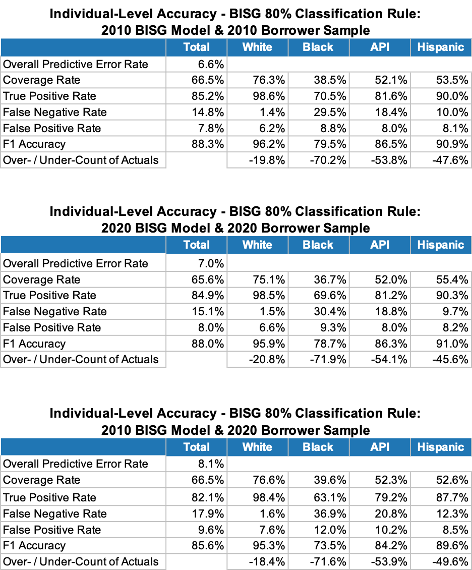
Figure 11 summarizes the BISG Models' individual-level predictive performance under the same three scenarios as described above. However, here I apply the BISG 80% classification rule instead of the BISG Max classification rule.
Overall, for BISG 80%-based individual-level race/ethnicity prediction, my analyses indicate that:
The general increase in racial/ethnic diversity between 2010 and 2020 causes the 2020 BISG Model's Overall Predictive Error Rate on the current borrower sample (the middle table) to be 0.4 percentage points higher (a relative increase of 6%) than that of the 2010 BISG Model on the 2010 borrower sample (the top table).
Relative to the BISG Max rule, the BISG 80% rule may appear far superior as a predictor of individual-level race/ethnicity as its 2020 overall predictive error rate is only 7.0% (middle table of Figure 11) versus 17.3% for the BISG Max rule (middle table of Figure 10). However, we need to remember that the BISG 80% rule is unable to classify an individual's race/ethnicity if none of his/her BISG probabilities is at least 80%. Accordingly, this classification rule does not achieve 100% sample coverage like the BISG Max rule; in fact, as shown in Figure 11 above, the rule only achieves a 65.6% average Coverage Rate on the 2020 borrower sample - which is 0.9 percentage points lower than that achieved by the 2010 BISG Model applied to the 2010 borrower sample. In terms of aggregate borrower counts (last row in each table), we see just how restrictive this classification rule is - with the number of Predicted Black adults only about 30% the size of actual Black adults, and similar large undercounts for other race/ethnicity groups. Overall, while those actual group members who can be classified are predicted more accurately; (1) almost a third of the entire sample cannot be classified, (2) the coverage rate actually falls further using the 2020 BISG Model on the current borrower sample (due to improved race/ethnicity diversity), (3) over 60% of Black adults cannot be classified, (4) those successfully classified have a slightly higher predictive error rate than in 2010, and (5) those who cannot be classified do not appear to be random - and, therefore, fair lending tests associated with the BISG 80% proxy groups may be biased.[16]
For current borrower samples, the 2010 BISG Model generates an even higher Overall Predictive Error Rate - i.e., 1.1 percentage points greater than the 2020 BISG Model (a 16% relative increase, see the bottom table). This occurs because the 2020 U.S. Census geo-demographic data is more aligned to the demographics of current borrower samples than the 2010 data.
In the next two sections, I explore how the 2020 BISG Model impacts fair lending disparity estimates using the same framework as my 2021 BISG Study.
6. 2020 U.S. Census Data: Impact on Disparate Treatment Disparity Estimates
As I wrote in my 2021 BISG Study,
"To assess the precise impact of the BISG proxies on the estimation of disparate treatment disparities, we first need a sample of lending outcomes in which the exact form and amount of the disparate treatment is known (i.e., the “ground truth”). To this end, and to avoid overcomplicating this analysis, we simulate a simplified disparate treatment scenario in which a certain minority group ... is charged a discretionary fee amount that is not charged to the corresponding White group – for example, a $100 “processing fee” is charged to Blacks ... but not to Whites. Given that we know the ground truth disparate treatment effect ($100), we can then assess whether the corresponding disparate treatment estimates produced by traditional fair lending testing tools on our synthetic dataset are biased in any way by our use of BISG-based proxies."
To update this analysis for the 2020 BISG Model, I performed the following:
I used my 2020 borrower sample to implement the disparate treatment scenario. For example, for the "Black Fee Only" scenario, I assigned all 2020 actual Black sample members a $100 fee and all other sample members a $0 fee.
To simulate typical fair lending analyses, I estimated the potential disparate treatment fee disparities using the 2020 BISG Model under both the "BISG Continuous" estimation approach as well as the "BISG Classification" estimation approach. The former employs a regression analysis framework in which each sample member's fee amount is the dependent variable and their corresponding set of BISG probabilities are the independent variables. For the latter estimation, I assume each sample member's race/ethnicity has been classified using either the BISG Max, BISG 80%, or BISG 50% classification rules.[17] Then, under each classification rule, each predicted group's actual fee amounts are averaged and the protected class fee disparities are directly calculated.
For each race/ethnicity group, I compare the predicted fee disparity amounts under the different estimation approaches to the actual (i.e., ground truth) fee disparity amount. The difference is expressed as a percentage and represents the estimated fee disparity bias caused by the inaccuracies of the BISG race/ethnicity proxies.
The estimated fee disparity biases for the 2020 borrower sample based on the 2020 BISG Model are compared to: (1) my original 2010 estimated fee disparity biases (i.e., using the 2010 borrower sample and the 2010 BISG Model) and (2) estimated fee disparity biases using the 2010 BISG Model on the 2020 borrower sample. The former helps to understand general bias changes over the past decade, while the latter indicates the impact of continued use of the 2010 BISG Model on current borrower samples.
These results are summarized below in Figure 12.

Based on these results, I note the following:
The first group of rows (“2010 BISG Model - 2010 Borrower Sample”) summarizes the results from my original 2010 BISG Study where - as discussed more fully there - the BISG Continuous estimation approach (last column) produced unbiased fee disparity estimates (i.e., 0% bias). The conditions for obtaining this result are similar to those discussed above in Section 4 (i.e., a borrower sample whose characteristics are statistically aligned with BISG Model's underlying Census data).[18]
Under the BISG Classification estimation approaches, on the other hand, we see that fee disparity biases are consistently negative ranging from a low of -8.6% to a high of -37.6% - with the BISG Max rule leading to the largest fee disparity underestimations, and the BISG 80% rule leading to the smallest underestimations. Again, the 2021 study provides further details on the drivers of these underestimations. However, in general, they are driven by both the False Negatives and the False Positives discussed in Section 5 above - with, for example under the "Black Fee Only" scenario, False Positive Blacks (with $0 fees) lowering the average estimated fee for Predicted Blacks below $100 and False Positive Whites (some with $100 fees) increasing the average estimated fee for Predicted Whites above $0.
The second group of rows ("2020 BISG Model - 2020 Borrower Sample") shows the results if we apply the 2020 BISG Model to current borrower samples. Again, since our current borrower sample characteristics are more closely aligned with the 2020 BISG Model's underlying data characteristics, the fee disparity biases under the BISG Continuous estimation approach are (effectively) zero. However, because of the general deterioration in the predictive power of the 2020 BISG Model for Black adults, the 2020 fee disparity bias magnitudes under the BISG Classification estimation approaches are generally larger than they were in my 2021 BISG study. Estimated disparity biases for Hispanics are the same or slightly lower than in 2010 while those for APIs are virtually unchanged.
Finally, the third set of rows ("2010 BISG Model - 2020 Borrower Sample") shows the results if one continues to use the 2010 BISG Model on current borrower samples. Here we see that - because the characteristics of the borrower sample are no longer statistically aligned with those of the 2010 BISG Model, the fee disparity estimates produced by the BISG Continuous estimation approach are no longer unbiased - although the magnitudes of the biases are relatively small (e.g., maximum of $3.50 on a $100 processing fee). Additionally, we see that the magnitudes of the disparity biases under the BISG Classification estimation approaches increase as well due to the general increase in False Positives and False Negatives (see Figures 10 and 11).
7. 2020 U.S. Census Data: Impact on Disparate Impact Disparity Estimates
In this final section, I explore how the revised 2020 BISG Model impacts traditional estimates of disparate impact. Similar to the prior section on disparate treatment, I adopt a simplified approach with known “ground truth” fee disparities in order to maximize insights. Specifically, I assume that disparate impact occurs when a lender charges a discretionary fee amount that varies with the general income level of the borrower. More specifically, I segment the current borrower sample into 10 deciles based on average 2020 CBG median income, and assume that fees are assessed according to the following discretionary fee schedule:[19]
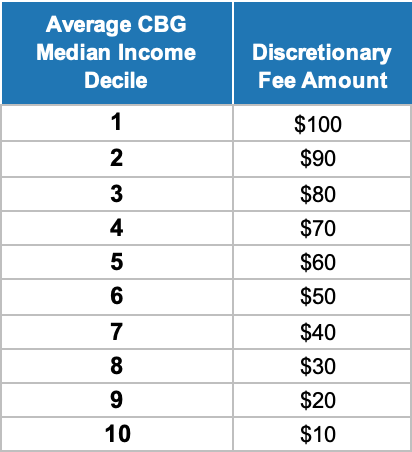
This scenario assumes that loan originators tend to charge lower income borrowers – regardless of their race/ethnicity – higher average fees, and higher income borrowers lower average fees. Importantly, disparate treatment is not present here since all borrowers within a given income range receive the same fee amount. However, because certain minority groups have lower average incomes than Whites, a disparate impact can be alleged - as illustrated below in Figure 13.
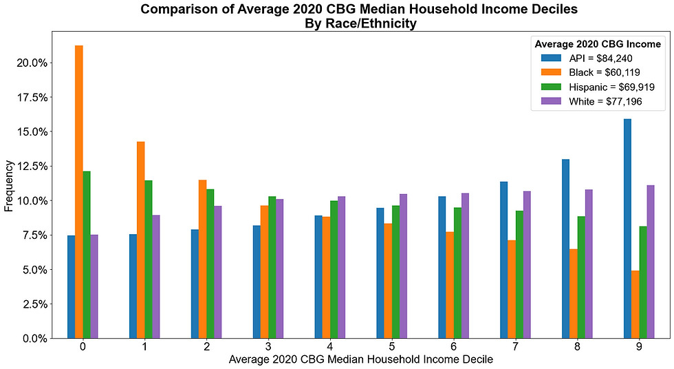
Here we see that Black and Hispanic borrowers have lower average 2020 CBG incomes than Whites (and APIs) due to a relatively larger concentration of such borrowers in the lower income deciles. According to our pricing scenario, this should cause Black and Hispanic borrower groups to exhibit higher average fee amounts than White (and API) borrower groups - leading to the disparate impact disparities as shown below.
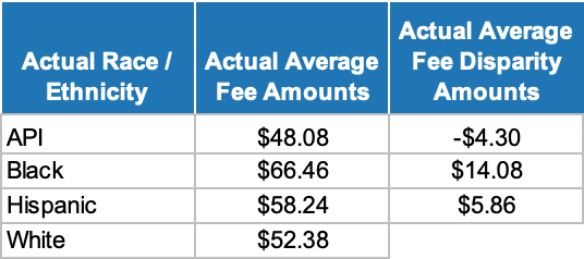
Figure 14 below presents the results of this disparate impact estimation scenario under alternative BISG proxy-based estimation approaches.
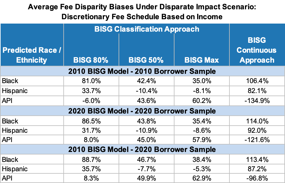
The first column of this table corresponds to the predicted group members being tested, the second through fourth columns correspond to the fair lending testing results under each of the three BISG classification rules used to predict the individual-level race/ethnicity of each group member, and the fifth column corresponds to the fair lending testing results using the BISG Continuous approach.[20]
Based on these results, I note the following:
The first set of rows (“2010 BISG Model - 2010 Borrower Sample”) shows the disparate impact disparity biases I estimated in my original study (i.e., using the 2010 BISG Model and a 2010 borrower sample). As that study noted,
"Overall, these results indicate that all BISG proxy approaches – including the BISG Continuous approach – yield biased disparate impact estimates even in the absence of any misalignment between actual and expected race/ethnicity distributions. In fact, these results indicate that the BISG Continuous approach yields the largest biases with magnitudes ranging from -135% for APIs to +106% for Blacks."
In general, and as I discuss further in my 2021 study, these disparities are inflated because the False Positives and False Negatives for each borrower group are not comprised of random group members. Rather, the False Negatives tend to be associated with higher income-lower fee "inside group" members, while the False Positives are associated with lower income-higher fee "outside group" members.
For example, the "Predicted Black" test group excludes a portion of Actual Blacks (i.e., False Negatives) and includes a portion of Non-Blacks (i.e., False Positives - most of which are White). However, when analyzing these two segments, one sees that the Black False Negatives have higher than average incomes - which means that their exclusion from the Predicted Black group increases its associated average fee amount. Alternatively, the predominantly White False Positive Blacks tend to have lower incomes - which means that they reinforce the elevated "Predicted Black" average fee amount. Additionally, since these White False Positive Blacks are excluded from the "Predicted White" test group, the remaining Whites will have a lower average fee amount. Both of these effects lead to an inflation in the estimated fee disparity amount between Black and White borrower groups.[21]
Moving down to the second group of rows ("2020 BISG Model - 2020 Borrower Sample"), we see that an updated 2020 BISG Model applied to a current borrower sample yields disparate impact disparity biases that are even more positive for Black borrowers. For example, under the BISG Continuous estimation approach, Black disparate impact disparity estimates are overestimated by 114% - a 7.6 percentage point increase from 2010 bias levels. The results for Hispanic and API borrowers are more mixed - with some biases larger and some smaller. However, I note that under the BISG Continuous estimation approach - which is the approach favored by the CFPB - the disparate impact disparity bias for Hispanic borrowers increases by almost 10 percentage points.
Finally, if disparate impact disparity testing on current borrower samples were based on the 2010 BISG Model, we see via the bottom three rows ("2010 BISG Model - 2020 Borrower Sample") that disparity biases under the BISG Classification approaches would generally be larger. However, interestingly, the disparity bias magnitudes under the BISG Continuous estimation approach would be slightly smaller than those based on the 2020 BISG Model.
A Couple of Final Thoughts
While the significant inflation in disparate impact disparity estimates may seem specific to my chosen scenario - i.e., based on relative income levels, it actually may not be. That is, I would also expect it to apply to disparate impact scenarios in which discretionary lender actions are based on other attributes that are correlated with borrower income. For example, if higher fees tend to be charged to borrowers with poorer credit, then a similar inflation in disparate impact disparities may arise since lower FICO scores tend to be correlated with lower income, and vice versa. That is, by excluding higher income Black adults (who may have higher FICO scores, on average) and including lower income White adults (who may have lower FICO scores, on average), a Predicted Black group may exhibit overestimated fees relative to Whites.
Finally, returning to the theme of model disparate impact, the 2020 U.S. Census data shows that the BISG Model's apparent adverse impact to minority group prediction accuracy - and their associated lending outcome estimates - deteriorates with the growing racial diversity of the U.S. population - particularly for Black Americans. This failure to identify accurately over 40% of Black adults, the exclusion of higher-income Black adults from the "Predicted Black" group, the inclusion of significant numbers of lower-income Whites to the "Predicted Black" group, the underestimation of Black disparate treatment disparities, and the overestimation of Black disparate impact disparities all contribute to the important question:
Why, in this day where algorithmic bias is a growing concern with predictive models, do we continue to use a model for fair lending compliance risk management that appears to show a growing algorithmic bias?
Some food for thought.
* * *
To learn more about Ric, read his bio here.
ENDNOTES:
[1] See, for example, "Fool's Gold? Assessing the Case For Algorithmic De-Biasing"
[2] See, for example, "Meta's Variance Reduction System: Is This the AI Fairness Solution We've Been Waiting For?"
[3] The "BISG Continuous" estimation approach - typically employed by the CFPB in its non-mortgage fair lending testing - is a disparity estimation methodology in which the sample borrowers' individual price metrics (e.g., borrower APRs, fees, dealer mark-ups, etc.) are regressed on the sample borrowers' corresponding sets of BISG continuous probabilities (i.e., no individual race/ethnicity classification is employed in this approach).
[4] The 2020 DHC File replaces the U.S. Census's 2010 SF1 File as the source of geo-demographic data for the CFPB's BISG proxy methodology. More detail can be found at the following link.
[5] Because my analyses are in the context of fair lending compliance risk management, I - like the CFPB - focus on the population of U.S. adults and exclude Puerto Rico (since the Census surname database - the other data source underlying the BISG Model - excludes Puerto Rico). Accordingly, the demographic trends presented in this section may differ from those produced by the U.S. Census Bureau and those contained in various media publications that focus on the Total U.S. population (i.e., adults and non-adults) inclusive of Puerto Rico.
[6] See "2020 Census Illuminates Racial and Ethnic Composition of the Country", U.S. Census Bureau, August 12, 2021.
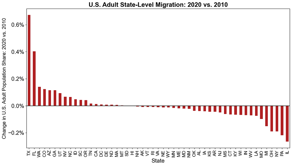
[7] Of course, these state-level migrations are heavily influenced by overall population migration trends during this 10-year period - as shown below.
[8] I note that for certain 2020 U.S. Census tables, the Census Bureau implemented a new differential privacy methodology to prevent the ability of users potentially to identify information about specific individuals - particularly in data stratifications that involve small numbers of individuals such as Census Blocks. Given this context, it is possible that the 2010-2020 demographic trends at the Census Block Group level presented in Figure 8 may contain results that are somewhat distorted by the impact of these adjustments. However, I note that - qualitatively - these results are consistent with the patterns observed at more aggregate geographic levels.
[9] Interested readers may wish to read the "Caveats and Future Efforts" section of my 2021 BISG Study (p. 10) for a discussion of the reasonability of my synthetic sample for these purposes. In particular,
Let us be the first to acknowledge that the synthetic sample used in these analyses may not be exactly representative of any lender’s non-HMDA customer base to which the BISG proxy model would be applied. Nevertheless, the synthetic sample does possess statistical properties – such as aggregate race/ethnicity distributions, correlations between “actual” and proxy races/ethnicities, as well as other accuracy measures – that are generally aligned with those measured in previous studies based on real world data samples. This provides a degree of confidence in the broad appropriateness of the synthetic sample for the goals set out above. However, the bias estimates generated from this sample should be considered “baseline” estimates associated with a broad geo-surname sample of the U.S. adult population.
[10] The mapping of 2010 U.S. CBGs to 2020 U.S. CBGs was performed using the U.S. Census Bureau's Block Group Relationship Files. In cases where a 2010 CBG was mapped to multiple 2020 CBGs, I selected the 2020 CBG with the highest population count. After this mapping, I was able to append 2020 CBG demographics for all but 924 (0.00924%) of the 10 million member 2020 synthetic borrower sample.
[11] Individual race/ethnicity prediction is used by some lenders as the basis for their fair lending disparity testing (instead of using the raw BISG probabilities in the BISG Continuous estimation approach). Additionally, most lenders have no practical alternative but to use individual-level race/ethnicity prediction when targeting transactions for manual follow-up review, or for selecting specific borrowers to receive customer remediation.
[12] As discussed more fully in the 2021 BISG study, micro-geographic segregation by race/ethnicity (e.g., at the census tract, census block, or census block group level) is one of the two sources of the BISG Model's predictive power - particularly for Black adults. Ironically, social progress in reducing residential segregation barriers - such as that observed in the 2020 U.S. Census data - also serves to reduce our ability to measure accurately potential fair lending disparities based on Census-based race/ethnicity proxy models.
[13] To be more precise, there are 1,137,542 Actual Black adults in my 2020 synthetic borrower sample. However, using the 2020 BISG Model and applying the BISG Max classification rule, only 647,553 of these adults are accurately identified as Black (i.e., 56.9% - the "True Positives" in the middle section of Figure 10) - indicating that 489,989 of Actual Blacks are misclassified as some other race/ethnicity (i.e., 43.1% - the "False Negatives" in the middle section of Figure 10). On the other hand, 915,480 sample members are predicted to be Black ("Predicted Blacks") which is -19.5% lower than the total number of Actual Blacks (i.e., the "Over-/Under-Count of Actuals" in the middle section of Figure 10). This means that 267,927 members of other race/ethnicity groups are misclassified as Black (i.e., 29.3% - the "False Positives" in the middle section of Figure 10).
[14] On its face, the Hispanic result appears somewhat counterintuitive since the 2020 BISG Model is more predictive for Hispanics, but - according to Figure 8 - Hispanics live in slightly more diverse neighborhoods. The reason both of these can be true is because: (1) the overall increase in the U.S. Hispanic population from 2010 to 2020 raised the Hispanic population share in 80% of CBGs - thereby increasing the predictiveness of the 2020 BISG Model for Hispanics, and (2) the re-distribution of Hispanics across CBGs since 2010 caused a shift toward relatively less segregated CBGs.
[15] As discussed in more detail on p. 27 of my 2021 BISG Study, F1 Accuracy is the harmonic mean of Recall Accuracy and Precision Accuracy. The former is measured as (1 - False Negative Rate), and the latter is measured as (1 - False Positive Rate). For example, using the 2020 BISG Model on the 2020 borrower sample, Black Recall Accuracy is 56.9% (= 1 - 43.1%) and Black Precision Accuracy is 70.7% (= 1 - 29.3%). As the harmonic mean is calculated as (2 * Recall Accuracy * Precision Accuracy) / (Recall Accuracy + Precision Accuracy), this yields a 2020 Black F1 Accuracy rate of 63.1% (= 2 * 56.9% * 70.7%) / (56.9% + 70.7%) - when calculated using higher precision.
[16] As discussed in my 2021 BISG Study, the Predicted Black borrower sample created by the BISG 80% rule is comprised of about 90% Actual Blacks (True Positives) - but markedly skewed to those who live in highly-segregated, lower-income geographies. They are supplemented by a small sample of non-Blacks (misclassified as Black, i.e., False Positives) who live predominantly in majority-Black, lower-income geographies. Accordingly, this skew creates a highly non-representative sample of Predicted Black adults with corresponding biases in fair lending testing results.
[17] The BISG 50% classification rule uses a >=50% BISG probability threshold to classify the race/ethnicity of a sample member.
[18] In an actual consumer lending context, it may be difficult to achieve the required alignment between sample and U.S. Census data characteristics - either because the lender does not have a broad, nationally-representative footprint, or because its customer base - while adults - are skewed toward higher-income or more creditworthy adults. If either of these is true, then it is unlikely that disparate treatment disparity estimates based on the BISG Continuous estimation approach will be unbiased. See pp. 75-79 of my 2021 BISG Study for further details.
[19] The median household income data is from the 2020 American Community Survey Census Block Group dataset and reflects a trailing five-year average (i.e., 2016-2020) expressed in 2020 dollars. For this data, see Steven Manson, Jonathan Schroeder, David Van Riper, Tracy Kugler, and Steven Ruggles. IPUMS National Historical Geographic Information System: Version 17.0 [dataset]. Minneapolis, MN: IPUMS. 2022. http://doi.org/10.18128/D050.V17.0. For sample members in CBGs with missing 2020 median household income data (about 4% of the sample), I used their 2010 median household income data - adjusted to 2020 dollars. Only 0.3% of the sample had neither 2010 or 2020 CBG median household income.
[20] Figure 14 is a summarized version of Figure 35 in my 2021 BISG Study (p. 84). I refer the interested reader to pp. 84-91 of that study for further details behind these bias estimates - as well as an intuitive discussion of their drivers.
[21] See pp. 84-91 of my 2021 BISG Study for a more detailed discussion of these effects - including specific numerical examples.
© Pace Analytics Consulting LLC, 2023.

