Unsafe and Unsound: A New Analysis of the CFPB's Use of BISG Race Proxies For Disparate Impact Enforcement

More than once now, the CFPB has deployed novel analytical technology in pursuit of an equally novel theory of discrimination without subjecting the tool to the same model validation discipline that federal regulators expect of the banks they supervise. This is the earlier—and costliest—case of this risk management failure: a proxy-based regression estimator that, under the disparate impact theory the agencies themselves pled, roughly doubled the pricing disparities behind more than $160 million in indirect-auto settlements, and then became a default test for many industry fair lending compliance programs.

Do As We Say, Not As We Sue ...

In April 2011, the federal bank regulatory agencies published detailed guidance on how supervised financial institutions ("FIs") should manage the key risks associated with the development, deployment, and ongoing use of quantitative models. Among other requirements, this Supervisory Guidance on Model Risk Management stressed the importance of rigorous independent validation testing of high-impact models to assess their conceptual and technical soundness for their intended purposes, as well as their predictive accuracy relative to known ground truths. It warned that unvalidated or unvetted models can create significant financial, operational, compliance, and reputational risks due to fundamental model errors, and the inappropriate use of an otherwise technically sound model "outside the environment for which it was designed."

"Even a fundamentally sound model producing accurate outputs consistent with the design objective of the model may exhibit high model risk if it is misapplied or misused. ... This is even more of a concern if a model is used outside the environment for which it was designed. ... Decision makers need to understand the limitations of a model to avoid using it in ways that are not consistent with the original intent. ... Limitations are also a consequence of assumptions underlying a model that may restrict the scope to a limited set of specific circumstances and situations." — Supervisory Guidance on Model Risk Management, April 2011.[1]

Within a few months after this model risk management guidance was issued, the Consumer Financial Protection Bureau ("CFPB" or "Bureau") opened its doors. The Bureau was not legally bound by this supervisory framework, but it soon began deploying advanced quantitative models against FIs that carried the very same risks the guidance was designed to mitigate. Two and a half years later, the Bureau and the Department of Justice ("DOJ") began extracting more than $160 million from four of the nation's largest indirect auto lenders—Ally, American Honda Finance, Fifth Third Bank, and Toyota Motor Credit—for alleged disparate impact discrimination in discretionary loan fees based on the outputs of these unvalidated quantitative models.

The evidence of this discrimination?

Statistically-estimated disparities in discretionary dealer mark-ups[2] across borrowers of different races.[3]

The novel technology?

The Bureau used two novel technologies to estimate these statistical disparities: First, because actual borrower race data were unavailable for auto loans, the Bureau used race proxies generated from a complex statistical methodology—Bayesian Improved Surname Geocoding ("BISG")—originally developed to investigate race-based differences in health plan quality.[4] Second, it used these estimated BISG race probabilities as predictors in a regression model (the Bureau's "BISG Continuous" regression model) to estimate dealer mark-up disparities for each racial group, interpreting the coefficients of these race proxies in the same manner as those estimated from ground truth race data.

The Bureau's fatal flaw?

It failed to understand the key risks associated with these race-based estimation methodologies. Its only publicly shared validation testing focused exclusively on the proxy methodology's calibration accuracy (i.e., its accuracy in predicting actual race). Yet, as I show below, it ignored a much more fundamental and critical model risk: whether its implementation of the BISG Continuous regression methodology was conceptually and technically sound for the Bureau's intended purpose. Specifically, the BISG Continuous regression methodology the Bureau adopted from the health services policy research area was developed to answer a very different question (disparate treatment) than the one the Bureau was asking of its FIs (disparate impact).

Under the very disparate impact theory the Bureau alleged, my validation testing shows that BISG Continuous produces fair lending disparities inflated by roughly a factor of two.[5] Therefore, the Bureau's failure to adhere to the same model risk management guidance as the banks to which its advanced technologies were applied was a double standard that inflicted the very harms the supervisory guidance was meant to mitigate.

And this regulatory double standard persists to this day. In fact, I have written extensively in my Fool's Gold series and in my Technological Exceptions article about the Bureau's more recent embrace and recommendation of complex, black-box "debiasing" technologies to mitigate credit model "disparate impact" without due consideration of several important model risks and limitations.[6] While the underlying advanced technologies used in these two supervisory areas differed, the risk management failures were largely identical: begin with a novel discrimination theory, adopt externally sourced advanced technologies to operationalize the theory, and give short shrift to the important validation testing that might reveal potential flaws in its intended use.[7]

This article makes the case that the Bureau's insufficient model risk management controls expose the financial industry to significant harm. As more evidence of this, I conduct the Bureau's missing conceptual and technical soundness validation testing of the BISG Continuous estimator, and show that its use of this methodology was plagued by significant flaws that should have been identified before deployment.

Let's dive in.

The Bureau's BISG-Based Indirect Auto Disparate Impact Measures

As described in my earlier article, Disparate Impact is Dead. Long Live Disparate Impact, shortly after the Bureau opened in 2011-2012, Director Cordray announced a formal commitment to use disparate impact liability in its ECOA fair lending enforcement—a position that federal bank regulators had rarely taken before the Obama Administration:[8]

"Consistent with other federal supervisory and law enforcement agencies, the CFPB reaffirms that the legal doctrine of disparate impact remains applicable as the Bureau exercises its supervision and enforcement authority to enforce compliance with the ECOA and Regulation B." — CFPB Bulletin 2012-04 (Fair Lending)

The target: Discretionary interest rate "mark-ups" that indirect auto lenders permitted their dealers to charge borrowers as compensation for certain loan application and origination services performed in connection with new- and used-car sales financing transactions.

The discrimination theory: The lender's "policy" of allowing dealers discretion to set the mark-up amount of each transaction created a disparate impact on certain demographic groups—such as Blacks, Hispanics, and Asians.

The results: Between December 2013 and February 2016, the Bureau and DOJ publicly announced four indirect-auto disparate impact pricing matters that became the defining federal actions of the industry-wide enforcement program totaling approximately $160 million in consumer redress and penalties:[9]

Table 1

The underlying legal theory was disparate impact; that is, the agencies did not allege that anyone directly priced loans based on the borrower's race. Instead, they alleged that the lenders' facially neutral policies, which allowed dealers the discretion to mark up the lender's buy rate, produced adverse statistical disparities in the average mark-ups paid by these demographic groups—effectively identifying the offending "policy" as the absence of one. While there is much to say about the Bureau's then-novel disparate impact discrimination theory, I set that discussion aside here—first because I've already addressed it in my Disparate Impact is Dead. Long Live Disparate Impact article and, more importantly, my focus in this article is the novel technology on which this novel discrimination theory ran.

As discussed previously, this novel technology was termed BISG—a statistical proxy methodology for identifying an individual's unknown race, developed by academic researchers to measure racial differences in health plan quality. Regression analysis was part of this line of research, with the authors using each individual's full set of BISG race probabilities in the regression model rather than converting them into a single predicted race indicator.[10] This regression analysis approach became known as "BISG Continuous" after it was deployed at the Bureau for indirect-auto fair lending testing.

While its academic research lineage was certainly important in establishing a baseline comfort with the BISG-based methodology, it was ultimately cold comfort, since the Bureau was applying it to answer a question quite different from the one for which the methodology was originally developed. While the health literature showed that the BISG Continuous method produced unbiased estimates of racial disparities in health outcomes that differed by race directly (i.e., disparate treatment), the Bureau adopted this methodology to measure racial disparities in lending outcomes under a theory whereby outcomes differed by race indirectly due to the differential effects of a facially-neutral policy (i.e., disparate impact). And over the course of a multi-year enforcement program, with dueling experts on every side and hundreds of millions of dollars at risk, the Bureau never wavered from its use of this novel technology, even though it was answering a different legal question than the one it was pleading. 

And, now, for those who just want the headline, it is this. There are actually two ways to use BISG probabilities to estimate traditional fair lending disparities accurately, and they are not two sides of the same coin. The choice of which to use depends critically on the underlying source of the racial correlation and, hence, on the legal theory of discrimination being asserted. The Bureau used the wrong one.

The Headline Result: There Are Two Disparity Estimation Methods, Each Accurate For Only One Type of Discrimination Scenario

Both BISG-based estimation methods start from the same place: each borrower's set of BISG race probabilities—for example, 70% Black, 20% White, 10% everything else. The fair lending analyst can then use these race probabilities to estimate a potential fair lending disparity in one of two ways:[11]

• Use them as race predictors in a regression. This was the Bureau's method. For the indirect auto disparate impact campaign, it used the raw probabilities as predictor variables in the BISG Continuous regression, with each borrower represented as partially Black, Hispanic, Asian/PI, and White. The resulting regression coefficients were interpreted as the potential fair lending disparity,[12] no different than if they had used each borrower's actual race identifier in the analysis. Even today, this method receives a formal academic endorsement as the "principled" estimator choice.[13]

• Use them as weights in an average. In this alternative estimation method, the analyst computes, for each racial group, a BISG probability-weighted average mark-up amount. For example, a borrower who is 70% likely to be Black contributes 70% of their mark-up to the Black group's average mark-up, 20% to the White group's average mark-up, and so on. Subtract the White weighted average mark-up from the Black weighted average mark-up, and you have the potential fair lending disparity. The same academic paper referenced above has largely dismissed this method as a "heuristic"— i.e., an intuitive shortcut without formal guarantees of consistency. And few lenders appear to use this fair lending disparity estimation approach.[14]

A regression versus a simple weighted average. In my experience, most analysts would overwhelmingly adopt the regression approach, as it's more efficient (i.e., it simultaneously tests all race groups) and consistent with the Bureau's historical approach. The problem is, it's not an either-or decision. As it turns out, each is accurate only under one type of discrimination scenario—either pure disparate treatment or pure disparate impact—thereby creating an identification problem for the fair lending analyst. The two methods produce estimates that generally bracket the true lending disparity, and the data alone generally cannot reveal where within that bracket the truth lies. The analyst needs to know the specific underlying legal theory of discrimination to select the appropriate measurement.

For those of you curious to know why, let me show you.

A New Validation Analysis of the BISG Continuous Method

First, A Quick Summary of My "Old" Validation Analysis

Five years ago, in my 2021 study, Modern Fair Lending Analysis: The Hidden Biases of BISG Proxy-Based Disparity Estimates, I built a synthetic borrower portfolio consisting of 10 million loans for exactly this purpose—a laboratory where the true race of every borrower is known so that every BISG-based disparity estimation method can be validated against the known ground truth. The BISG race probabilities were perfectly calibrated by construction, so any errors that emerged would not be due to bias in the BISG probabilities. And within this synthetic portfolio, I controlled the discrimination scenario—assigning discretionary fees either directly based on the borrower's true race (disparate treatment) or indirectly based on a socioeconomic factor correlated with race (disparate impact).[15]

For my disparate impact validation analysis, I assigned a discretionary fee based on each borrower's income, assumed to be equal to the U.S. Census Bureau's median income for the Census Block Group ("CBG") where the borrower resided. Borrowers in the top income decile of all U.S. CBGs paid a $10 fee, borrowers in each decile down paid $10 more, and borrowers in the bottom decile paid $100. Race had no direct impact on the borrower's fee.  In fact, all borrowers within a CBG received the same fee regardless of their race. In this scenario, fees differed by race for one reason only: Black and Hispanic borrowers, on average, were concentrated in lower-income CBGs relative to White borrowers. Therefore, a facially neutral, income-based fee policy caused a racially skewed pricing outcome—a textbook disparate impact scenario.

For my current validation analysis of the Bureau's BISG Continuous method, I extracted a 10% random sample from my 2021 synthetic borrower portfolio (i.e., 1 million borrowers) to compare the two BISG-based estimation approaches above, both with each other and against the known ground truth disparate impact ("DI") disparity.[16] The results of these comparisons are summarized below.

Table 2

As shown in this table, the "principled" BISG Continuous regression model used by the Bureau actually doubles the underlying true DI disparity for Blacks—yielding an estimate of $31.40, compared with the known true disparity of $15.09.[17] Alternatively, the academically dismissed "heuristic" weighted average estimation method misses the true DI disparity by only six cents. And this was not a quirk of one racial group. Across all groups tested (Black, Hispanic, and Asian), the BISG Continuous regression method overstates the true DI disparity by 82% to 134%, whereas the weighted average method remains within 0.4% of the truth.

For those who may be wondering: No. This estimation bias cannot be attributed to a small sample or to an imperfectly calibrated racial proxy. The sample contained one million observations (10% of the population), the laboratory sample's true races were intentionally calibrated to the BISG proxy probabilities, and the weighted-average estimator produced nearly dead-on DI disparities for each racial group. The bias arose because an estimator created for one type of discrimination scenario was being asked to measure another. The original BISG regression method implicitly presumed disparate treatment, in which race directly affects outcomes. The Bureau's scenario is disparate impact, in which race affects outcomes (i.e., fees) indirectly through a chain running from race to geography to income to fees, which is much different.[18]

Shouldn't the Bureau have known this?

Yes. But, ironically, it may not have been considered, as the Bureau pled a novel disparate impact theory of discrimination that failed to identify the specific mark-up policy rule (other than "discretion") responsible for the alleged adverse effects on racial minorities. Had the Bureau pled a more specific causal policy—for example, that mark-up variability was largely tied to differences in income or credit quality—the underlying econometric assumptions necessary for an unbiased and consistent estimator could have been more easily identified and tested by Bureau economists. No one involved in the estimation—not the Bureau's economists, nor the lenders' experts—ever had the context to ask whether the estimator was conceptually sound under the Bureau's own theory of the case, because that theory was never explicitly stated.[19]

Now that we have the broader context, I will show how this bias arises in a pure disparate impact scenario, and how the alternative "heuristic" estimator (the weighted average) eliminates it.

My New Validation Analysis

Let's start with a very simple but powerful example that reveals the precise mechanism behind BISG Continuous's inflated DI disparity estimates. For my non-technical readers, while this narrative uses some mathematical expressions, I have kept the math to a minimum (in the realm of introductory statistics) to provide a simpler, more intuitive explanation of the results.

To begin, consider a lender that purchased 200 closed auto loan contracts from a dealer primarily operating in two geographic neighborhoods. 100 of these borrowers resided in a low-income neighborhood ("Neighborhood L") and 100 resided in a high-income neighborhood ("Neighborhood H"). For simplicity, I assume the dealer charged all borrowers in the low-income neighborhood a discretionary fee of $100 and charged no discretionary fee to borrowers in the high-income neighborhood ($0). I also assume, again for simplicity, that there are only two races—Black and White, with Neighborhood L exhibiting a greater concentration of Black residents and Neighborhood H exhibiting a greater concentration of White residents.

The table below summarizes this simplified disparate impact scenario:

Table 3

The Ground Truth DI Disparity

If the lender knew the underlying race of each borrower, it could directly calculate the "ground truth" DI disparity.

• The 100 Black borrowers were charged an average fee of $70 = (70 × $100 + 30 × $0) ÷ 100

• The 100 White borrowers were charged an average fee of $30 = (30 × $100 + 70 × $0) ÷ 100.

• The true underlying Black DI disparity is $40—and it is real. Black borrowers genuinely paid more than White borrowers due to the groups' different locations under a geography-correlated, facially-neutral fee rule.[20]

The Bureau's BISG Continuous Disparate Impact Disparity Estimate

As with all non-HMDA loan products, the lender would not have access to each borrower's true race. Instead, let's assume it adopts the Bureau's BISG Continuous regression framework to analyze the statistical evidence for a potentially illegal Black DI disparity. Specifically,

For each of the 200 borrowers, the lender calculates the following set of BISG race probabilities based on the U.S. Census racial demographics of each neighborhood (excluding surname, for now):

Table 4

The lender then uses the Black BISG probability as the predictive factor in an OLS regression of each borrower's discretionary fee amount. The White probability is omitted from the regression per standard practice.

In this OLS regression equation, Y is the discretionary fee charged to each borrower, BISG-B is each borrower's BISG black probability per the table above, and β is the estimated DI disparity for Blacks relative to Whites.[21]

Applied to the lender's loan portfolio of 200 borrowers, this BISG Continuous regression yields an estimated β of $250—more than six times the $40 ground truth Black DI disparity calculated above.

Let's sit with that for a moment.

The innovative technology the Bureau adopted to bring numerous multimillion-dollar enforcement actions and MOUs across the indirect auto lending industry produces highly biased DI disparity estimates, and all it takes is a simple toy example to see this.

While some may find this result surprising, I note that it is consistent with the findings of my 2021 study The Hidden Biases of BISG Proxy-Based Disparity Estimates (discussed in the prior section), which used a much larger synthetic loan portfolio to analyze this issue.

So what's new here?

In my 2021 study, my explanation of the source of this bias was ultimately unsatisfying because it was framed in terms of a mathematical expression that lacked intuition. Additionally, while I identified specific alternative estimation techniques that eliminated this bias (i.e., bootstrap / proportional regression), the conceptual link between these methods and the source of the bias eluded me.

Those gaps are now closed, and the answers that emerge bring a newfound clarity to how BISG-based fair lending testing should be implemented to obtain unbiased results.

Let's dig further.

The Root Cause of BISG Continuous's DI Disparity Inflation

To investigate the root cause of this Black DI disparity inflation result, I start with how the OLS regression model calculates the Black DI disparity when the borrowers' true races are known:

In this OLS regression model, Black is now an integer variable representing each borrower's true race—taking the value 1 if the borrower is Black and 0 if the borrower is White. Y is still the discretionary fee charged to each borrower, and β is now the ground truth DI disparity between Blacks and Whites.

The Black ground truth DI disparity, β, is calculated mathematically as:

where:

• Cov(Y, Black) is the covariance between the borrowers' discretionary fees and their true race. Conceptually, it measures how the two move together—positive values indicate that Blacks tend to experience higher fees than Whites, and negative values indicate the opposite. In my example, this covariance term equals $10.00—a positive value indicating that, in the aggregate, Blacks exhibit higher fees than Whites, consistent with the fee policy rule that charges higher fees to borrowers with lower incomes, and with the concentration of Black borrowers in lower-income neighborhoods.

• Var(Black) represents a numeric measure of the racial variability of this borrower population. Low values (e.g., 0.0475) indicate that the overall borrower population is relatively racially homogeneous (e.g., 95% White and 5% Black). In contrast, high values (e.g., 0.25) indicate that the borrower population is relatively diverse (e.g., 50% White and 50% Black). In our example, this variance term is equal to 0.25— reflecting a high degree of racial diversity in the overall sample (i.e., 50% Black and 50% White).

• β = $10.00 / 0.25 = $40, which is exactly the ground truth Black DI disparity amount we directly calculated previously.

This example demonstrates that the BISG Continuous methodology can produce accurate ground truth DI disparity estimates when the true race is known. So the bias problem is not an inherent flaw in the regression methodology itself. It arises with the use of the BISG probabilities as race proxies. To investigate this, let's perform one final mathematical step to see how substituting BISG race probabilities into the OLS regression framework affects the Black DI disparity estimate.

Because the BISG proxy methodology uses U.S. Census demographic data at a geographic level (e.g., zip code, census tract, census block group), the β calculation can be usefully disaggregated into the following two geographically-based sub-components: (1) the within-geography effect and (2) the between-geography effect.

Using the laws of total variance and covariance, the β estimation equation in (3) can be decomposed into the following equivalent estimation equation:

This shows that the Black DI ground truth disparity β equals the weighted average of the between-neighborhood and within-neighborhood Black DI ground truth disparities, where the weight on each geographic estimate equals that geography's share of the portfolio's total racial variability. Specifically, V equals the "between geography" share of the portfolio's total racial variability and 1 - V equals the "within geography" share.

In our two-neighborhood example, V can be calculated using a simple one-way analysis of variance ("ANOVA") of borrower race on the two neighborhood components as shown below.

Table 5

Here we see that only 16% of the portfolio's total racial variation lies between the neighborhoods. Intuitively, this reflects the relatively modest degree of racial segregation (i.e., Neighborhood L is 70% Black, Neighborhood H is 30% Black, and the overall population is 50% Black).  The other 84% of the portfolio's racial variation occurs within the neighborhoods, capturing individual racial differences relative to the neighborhood average (e.g., Neighborhood L where 70% of borrowers have a true race value of 1 and 30% of borrowers have a true race value of 0 vs. a neighborhood average race value of 0.7).

At the most extreme level of segregation—that is, if all Black borrowers lived in Neighborhood L and all White borrowers lived in Neighborhood H—V would be equal to 1, since there would be no racial variation within either neighborhood. All racial variation occurs between neighborhoods. Alternatively, if each neighborhood reflected the same racial diversity as the overall population (i.e., 50%), then V would equal zero due to the complete lack of neighborhood segregation. All racial variation in the portfolio would occur within neighborhoods where half the borrowers are Black and half are White.

With this 0.16 value of V, I can now rewrite equation (4) as:

where:

• β Between = $250, which represents the results of the fee regression when the neighborhood black share is used as the predictor variable (i.e., 0.70 for individuals residing in Neighborhood L and 0.30 for individuals residing in Neighborhood H).[22]

• β Within = $0, which represents the results of the fee regression when the individual borrower's actual race is used as a predictor after holding the borrower's neighborhood fixed. This estimate is zero for the current portfolio because all borrowers in a neighborhood pay the same fee regardless of their race, since their incomes are assumed to be the same.

• β = $40—consistent with the ground truth disparity calculated above. This demonstrates the accuracy of the ground truth decomposition.

OK, so what happens when the lender uses BISG probabilities as proxies for true race?

Since the BISG proxy methodology uses geographic-level demographic data (i.e., neighborhood racial compositions), each probability effectively operates as a myopic lens that only sees the borrower's race at the neighborhood level, not the individual's racial identity within it. For example, each of the 100 borrowers residing within Neighborhood L receives the same BISG race signal (70% Black, 30% White) even though each resident is either Black or White. By blurring individual racial identities within neighborhoods, BISG fails to account for the within-neighborhood variation needed for accurate DI disparity estimation per equation (4) above. Of course, adding surname information sharpens the lens primarily for Hispanics and Asians; however, for this analysis, I focus only on geography to make the mathematics and intuition clearest. Surname effects will be incorporated further below.

Using our neighborhood-level BISG probabilities as predictors in the BISG Continuous regression expressed in equation (1), I now obtain the following version of the β decomposition expressed in equation (4):

Unlike the true-race version expressed in equation (5), all racial variation now occurs between geographies rather than also within them, since BISG cannot "see" racial detail within neighborhoods. In the absence of this within-neighborhood racial variability, V equals 1, and the Black DI disparity estimate under BISG Continuous equals $250.

Let's take in what this means intuitively for the resulting Black DI disparity estimate.

Because BISG cannot "see" the additional racial variability that exists within each neighborhood, BISG Continuous discards 84% of the total racial variability in our sample (see Table 5 above). And as we saw in equation (5), this discarded information is critical for an accurate Black DI disparity estimate.

Specifically, BISG Continuous doesn't "see" the 30 Black borrowers in Neighborhood H that received the same $0 fee as their White neighbors, or the 30 White borrowers in Neighborhood L that received the same $100 fee as their Black neighbors. Therefore, its myopia fails to "see" the zero fee disparity that actually exists within each neighborhood. Since the overall BISG Continuous Black DI disparity is a weighted average of the between-neighborhood and within-neighborhood fee disparities, excluding the $0 within-neighborhood disparity prevents BISG Continuous from recovering the ground truth portfolio Black DI disparity of $40.

This analysis also reveals that the size of this estimation bias depends critically on the true underlying value of V, which I refer to as the "segregation index".[23] In general,

• Higher V values (i.e., more neighborhood segregation) mean that BISG Continuous discards relatively less "within neighborhood" disparity information, meaning there is relatively less DI disparity bias. Alternatively, lower V values (i.e., more neighborhood integration) mean BISG Continuous discards relatively more of the "within neighborhood" disparity information, thereby causing more DI disparity bias.

• At the extremes: V = 1 (i.e., complete segregation), the BISG Continuous DI disparity exactly matches the ground truth DI disparity, as no useful information is excluded (i.e., all racial variation is between neighborhoods). However, as V falls toward zero, the DI disparity overstatement grows without bound as more and more useful DI disparity information is discarded by BISG's myopic racial lens. Perhaps counterintuitively, BISG Continuous is most biased precisely where a compliance officer would feel safest: in diverse, integrated neighborhoods (i.e., where the racial distribution aligns with that of the overall population).

Given these results, the natural next question is:

What about disparate treatment discrimination? Is BISG Continuous equally biased when used to measure disparities under a discrimination scenario in which lending outcomes vary directly by race?

Interestingly, the answer is No.[24] And the reason can be proven using the same analytical framework above.

Why BISG Continuous Produces Accurate Disparate Treatment Disparities

For my disparate treatment scenario, I use the same example of two neighborhoods, each with 100 borrowers. However, this time the lender's dealer discriminates against Black borrowers by charging each a $100 fee while charging each White borrower no fee ($0), yielding a Black disparate treatment ("DT") disparity of $100.

Under this scenario, the β decomposition equation (4) using true race would yield the following.

Notice that V is unchanged relative to its value in the DI analysis above, since it depends only on the portfolio's geographic racial distribution, not on the discrimination scenario. What changes under disparate treatment is that the between-neighborhood and within-neighborhood disparity estimates are now identical, a natural result of pricing based on individual race rather than geographically correlated socioeconomic factors. Fees follow the individual, not the geography—wherever Black and White borrowers are present, the Black disparity will always be $100.

Now, assuming true race is unavailable to the lender, our β decomposition analysis changes to the following:

As before, since BISG cannot "see" individual races within neighborhoods, it effectively discards all within-neighborhood DT disparity information and bases its overall Black DT disparity estimate solely on between-neighborhood DT disparity information. However, under disparate treatment, where fees follow the individual, discarding this information has no effect on the model's estimated Black DT disparity, since the within- and between-neighborhood DT disparities are identical. BISG Continuous discards data with no incremental predictive power, thereby yielding an unbiased DT disparity estimate.

Summarizing My Validation Testing: The BISG Continuous Bias Rule

The results above can be summarized as a single overall BISG Continuous Bias Rule for both discrimination scenarios. Using the β decomposition equation (4) under both the true race and the BISG Continuous methods, subtracting one expression from the other, and rearranging the terms yields a single rule about BISG Continuous disparity bias:

According to this rule, BISG Continuous's disparity bias depends on three factors:

• The underlying disparity between neighborhoods: β Between

• The underlying disparity within neighborhoods: β Within

• The segregation index, V

The first and second factors—i.e., the gap between the between-neighborhood and within-neighborhood disparity estimates — determine whether bias exists at all. At a conceptual level, it reflects the underlying discrimination legal theory expressed in mathematical form: pure disparate treatment sets the gap to zero under the constant-surcharge scenario modeled here since the two disparities are identical, whereas pure disparate impact creates a nonzero bias amount for reasons discussed previously.

Whether the disparate impact bias is positive or negative depends on whether the facially neutral, geographically-correlated "policy" channel burdens or benefits minority neighborhoods. In the current example, the fee policy operates entirely at the neighborhood level, since residents' incomes within each neighborhood are assumed to be the same. As fees are higher for lower-income neighborhoods, and Blacks are more likely to live in lower-income neighborhoods, β Within = 0 and β Between > 0, and the Black DI disparity bias is positive.

Must lender policies operate explicitly at the geographic level for this result to hold?

No—they can operate at the individual level, but the socioeconomic factor they price on must satisfy two conditions: (1) it varies across geographies in step with racial composition—that is, high-minority areas sit systematically on the disadvantaged end of the factor and (2) whatever variation the factor has within a geography is unrelated to race—that is, neighbors of different races look alike on it.

What do these two conditions mean in practice?

Let's test them with a small change to the toy example. Suppose the dealer prices each loan on the borrower's own income (not the neighborhood's median income). On its face, this seems like a very different policy—every borrower now receives an individually determined fee. But what has actually changed from BISG's perspective? Nothing. Within each neighborhood, incomes now differ from borrower to borrower, but—by condition (2)—those differences are unrelated to race. Two neighbors of different races with the same income pay the same fee. So the new borrower-level variation carries no racial signal at all. It simply adds noise to the fees. Meanwhile, all of the racial differences in income still sit exactly where they sat before—between the neighborhoods, with lower incomes and higher fees concentrated in the neighborhoods where minority borrowers live. And between the neighborhoods is precisely where BISG looks. Run the regression, and the estimated disparity comes back inflated by essentially the same factor as before because the bias depends not on the level at which the policy operates, but on where the socioeconomic factor's racial correlation lives.[25]

The third factor, (1 - V), reflects the share of total racial variation that the BISG Continuous model discards. It acts as an amplifier term. That is, for a given difference in disparities between and within neighborhoods, the degree of bias varies directly with the share of total racial variation within neighborhoods that BISG discards. The discard is harmful only because, under my disparate impact scenario, the discarded evidence would have disagreed: within a neighborhood, borrowers of different races face the same fees, so the within-neighborhood variation indicates no disparity at all, while the between-neighborhood variation, carrying the full weight of the disparity estimation, indicates a large one. BISG Continuous "sees" only the second disparity and assumes it is representative of all the racial variation—including the share it never saw, where the disparity is actually zero.

Does The Bias Rule Hold in More Realistic Data?

Clearly, my two-neighborhood example is highly stylized: I chose its numbers and assumptions to make specific points. So let’s take the bias rule back to my one million synthetic borrower sample, where the number of neighborhoods is in the tens of thousands, and the racial geography is the actual U.S. Census geography.

According to the rule in equation (9), under pure disparate impact, β Within = 0 and BISG Continuous's relative DI disparity bias should equal one divided by the segregation index, derived as follows:

Relative DI disparity bias does not depend on the size of the fee, the size of the disparity, or anything else about the lender’s conduct—it depends only on the segregation index, which reflects the relative importance of the within-geography racial variation discarded by BISG Continuous.[26] For example, in my simple example above:

• Relative Bias = 1/0.16 = 6.25, reflecting the fact that BISG Continuous discarded 84% of the racial variation (1 - V) due to BISG's racial myopia.

• This Relative Bias prediction based on V exactly matches the ratio of Black DI disparities under BISG Continuous and true race: $250/$40 = 6.25.

For my one million synthetic borrower sample, a Relative Bias prediction under the same income-based fee policy rule can be computed simply from V values derived from the racial composition of the samples' Census Block Groups ("CBGs"). I then compare these Relative Bias predictions with the true Relative Bias values, calculated from the samples' BISG Continuous DI disparities relative to the known ground truth DI disparities, to assess their accuracy. The table below shows this comparison and, importantly, also includes the effect of borrower surname to see how its inclusion impacts my analysis:

Table 6

The first column lists the specific subsamples analyzed by both portfolio geography and race. I include all three race proxies—Black, Hispanic, and Asian/PI, as well as both national and local portfolios. The second column contains the segregation index, V, for each sub-sample calculated directly from the U.S. 2020 Census race and population data at the Census Block Group level. The third column calculates the Predicted Relative Bias of BISG Continuous's DI disparity using only my 1/V rule. The fourth column presents the Actual Relative Bias of BISG Continuous's DI disparity, using DI disparity estimates from the BISG Continuous model relative to the known ground truth; importantly, the BISG probabilities used in the fourth-column estimates are based only on borrower geography (same as in my simple example above). The fifth column presents the same Relative Bias estimates, but this time using "full" BISG probabilities that include both borrower geography and surname. Finally, the sixth column calculates the "Surname Benefit," which is the share of the geography-only bias (Relative Bias in excess of 1) eliminated by the surname input: e.g., Hispanic, (1.73 − 0.49) / 1.73 = 72%.

Three main conclusions follow from these results.

• First, the bias rule is confirmed in more realistic data. It is structural, not a statistical artifact.  As shown in the fourth column, using the BISG geography-only proxy, the Relative Bias calculated with the BISG Continuous model, relative to known ground truth, matches 1/V essentially exactly for every sub-sample. The 200-borrower example sits on the same curve: its 70/30 composition yields V = 0.16 and a Relative Bias of 6.25×, while the national Black figure lands where its own segregation index places it—V = 0.51, an overstatement of 1.98×. One rule, many different-looking numbers, each predicted exactly as shown in this chart.

  

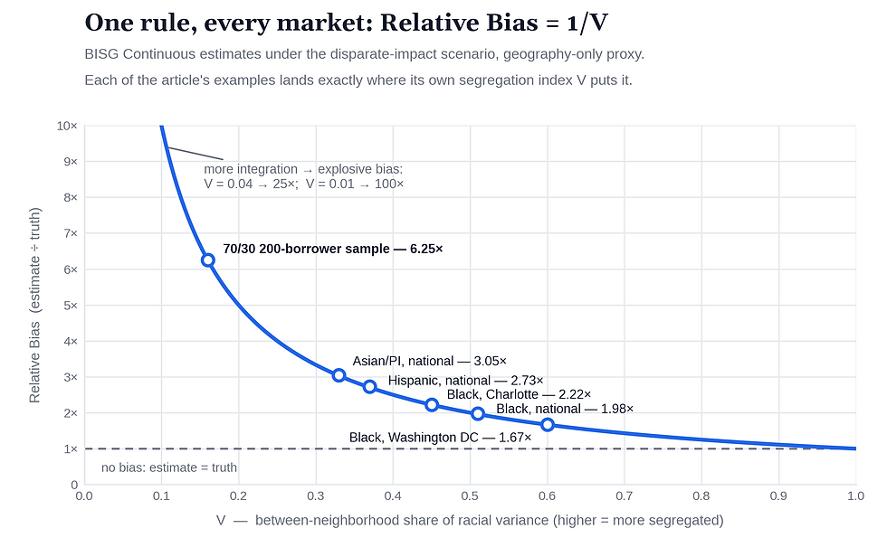
  Figure 1

  And note the direction: my simple example's neighborhoods are considerably more integrated than the national block-group geography, and its overstatement is correspondingly worse—this is the amplifier logic in action.

• Second, the inclusion of surnames mitigates the groups you would expect, but not the group with the most focus. Surnames restore part of BISG's vision of within-neighborhood racial variability that geography alone obscures. But this benefit is impactful only where surnames are racially distinctive, i.e., for Hispanic and Asian borrowers, for whom surname information removes roughly three-quarters of the geographic-only bias. However, for Black borrowers whose surnames largely overlap with White surnames, surnames remove only about 5% of the geography-only bias, leaving Black borrowers with the highest national-level DI disparity biases under BISG Continuous (1.93x vs. 1.49x for Hispanics and 1.47x for Asians). The group at the center of most disparate impact reviews and of all four of the agencies' indirect auto-lending fair lending enforcement actions is the group that surname benefits least.

• Third—and this is the conclusion I most want to emphasize—the bias was predictable in advance, from public data, with no outcome data at all, only the portfolio's geographic footprint and public Census files.  V is computed from U.S. Census racial compositions alone. It does not depend on the lender, the product, the fees, or the outcome being tested. Anyone validating the BISG Continuous method for disparate impact use in 2013 could have computed the segregation index for the relevant portfolio geography, taken its reciprocal, and known that a BISG-driven disparity would come back roughly doubled for Black borrowers. The validation exercise this article has walked through required 200 hypothetical borrowers, introductory statistics, and the U.S. Census Bureau’s public files. That is what makes this omission a risk management failure rather than a technical one. All they needed to find this flaw was a standard model validation review of the method's conceptual and technical soundness, no different than what federal bank regulators expected of their supervised institutions.

What About the Charlotte and DC results?

I included the last two rows of the table for Washington, DC, and Charlotte, NC to make some important points about national vs. market-level DI disparity bias results.

• DI disparity bias under BISG Continuous is footprint-specific, not a national constant. The 1.98× national figure applies to a nationally representative book of business. A real lender’s Relative Bias will reflect the specific segregation index of its own borrower footprint, as shown for the two sample markets in the bottom two rows—1.67× in DC and 2.22× in Charlotte, both for Black borrowers. Different lending footprints not only produce different Relative Biases in DI disparities calculated for the same demographic group, but also affect the comparability of lenders' fair lending performance for the same racial group.

• Integration makes the bias worse, not better. Recall the counterintuitive result from the two-neighborhood example: integration makes the DI disparity bias worse. The two metro rows drive this point home using real cities. Washington, DC is among the most residentially segregated markets in the country (V = 0.60), and the BISG Continuous model inflates the DI disparity there by “only” two-thirds. Charlotte—the comparatively integrated market (V = 0.45)—more than doubles it (2.22×). These results demonstrate that BISG Continuous is most reliable in the most segregated markets and least reliable in diverse, integrating markets.

• Even the surname benefit is a function of geography. The Black-borrower benefit is 4% in DC but 23% in Charlotte—and not because Charlotte’s surnames are any more racially distinctive. In an integrated market, BISG Continuous discards more within-neighborhood racial detail, so the same modest surname signal has more discarded information to recover. While the surname input helps most exactly where the problem is worst, it is still not enough—Charlotte’s 2.22× DI disparity bias falls only to 1.94×, essentially the national figure.

What About Disparate Treatment Scenarios?

Table 7 below presents the same results for the laboratory's disparate treatment scenario in which all members of the minority group are charged $100 while White borrowers are charged $0—creating a ground truth DT disparity of $100.

Table 7

Under a disparate treatment scenario, V no longer impacts BISG Continuous estimation bias since 𝛃 Within = 𝛃 Between, and Bias therefore equals zero per equation (9). Accordingly, I predict BISG Continuous to produce unbiased DT disparity estimates (i.e., Relative Bias = 1), and that is what I find in these results—along with something else that's very interesting.

In the fifth and sixth columns, unlike the results from the disparate impact scenario, we can see that adding surname demographics to the BISG probabilities has no meaningful impact on the measured bias—particularly for Hispanic and Asian/PI groups for whom the surname benefit was greatest in Table 6. The very small reductions I obtain are driven by the demographic drift associated with using national surname demographic data at the CBG level.

So How Should Pure Disparate Impact Disparities Be Measured When True Race is Unknown?

Thankfully, the analyses above suggest a solution. The BISG Continuous regression fails to produce accurate DI disparity estimates because the neighborhood-level BISG probabilities cannot "see" the within-neighborhood racial variability needed to properly offset the observed between-neighborhood fee differences. Disparate treatment disparities under BISG Continuous suffer from the same information exclusion. However, because fees are individual-specific, the within-neighborhood disparity is the same as the between-neighborhood disparity, with no practical impact on the resulting regression estimate.

For pure disparate impact, we need an estimator that is unaffected by this BISG-driven information loss. The answer, which may be surprising to some, is the simple difference between races in weighted average fees—i.e., the “heuristic” estimator described at the beginning of this article.

Specifically, for each race group r, compute the BISG probability-weighted average of the borrowers' (i) fees, and take differences from White:

Weighting every borrower's fee (Y) by their probability of being Black (BISG-B) and dividing by the total estimated number of Blacks (i.e., the sum of BISG-B's) yields an average Black fee for the whole BISG-proxied Black portfolio population. Substituting BISG-W in this equation and performing the same calculations yields the portfolio's average White fee. None of the discarded information plaguing BISG Continuous occurs with this BISG-based headcount approach.[27]

Using the BISG probabilities as weights for the fees means that borrowers in heavily Black neighborhoods contribute a lot to the average Black fee, while borrowers in heavily White neighborhoods contribute almost nothing. The reverse is true for the average White fee. Provided the BISG probabilities are accurately calibrated—i.e., a borrower assigned a 70% probability really is Black 70% of the time, neighborhood by neighborhood—this probability-weighted population will have the same neighborhood mix as the actual Black population.[28]

Now, let's apply this alternative methodology to my small 200-borrower example and see how it works.

• The Black-weighted average fee is equal to ($100 x 70 + $0 x 30) / 100 = $70.

• The White-weighted average fee is equal to ($100 x 30 + $0 x 70)/100 = $30.

• The Black DI Disparity = $70 - $30 = $40, which is the ground truth Black DI disparity, exactly.

No variance or covariance term ever enters the calculations, so BISG's discarded information has nothing to distort. 

Next, I apply the weighted-average DI disparity estimator to the 1 million national sample from my 2021 study. The results are summarized in the table below:

Table 8

When geography-only BISG probabilities are used as the weights in the weighted average estimator, the resulting DI disparity estimate matches the ground truth DI disparity estimate exactly for each geography-race sub-sample. With full BISG probabilities that include surname demographics, the results are very similar, though there are minor discrepancies reflecting calibration drift. That is, because the surname information is calibrated nationally, not locally, the probabilities place slightly too many estimated Black borrowers in some neighborhoods and too few in others—an error the geography-only weights cannot make, since they are matched to each census block group's actual composition by construction.[29]

Astute readers of my 2021 BISG research study might recognize that this alternative weighted average DI disparity estimator is a simpler version of the two alternative BISG-based DI regression methodologies I proposed there.

• Proportional Regression—a weighted least squares regression of fees on race indicator variables, where the BISG probabilities serve as observation weights. The coefficients on the race indicator variables reproduce the simple weighted average DI disparity exactly.[30]

• Bootstrap Regression—this method repeatedly samples a definite race for each borrower from their underlying BISG probabilities, re-estimates the DI disparity on each sample using OLS regression of fees on the sample's definite races, and averages the disparity estimates across samples. As my 2021 study proved, this estimation process converges to the simple weighted-average DI estimate exactly.

As I wrote in 2021, both approaches work for the same underlying reason: they “move the uncertainty of race/ethnicity membership out of the regressors—thereby eliminating the cause of the bias.”  However, as the above analysis has shown, regression models are not actually needed for accurate DI disparity estimates—a simple difference in weighted averages can suffice. Where these more complex approaches may be useful is when you need confidence intervals, significance tests, or when control variables become important.

But let's not lose sight of the asymmetric performance of these estimation methodologies according to these analyses. In a pure disparate treatment world, this weighted-average estimation methodology fails.

• Run the weighted average on the 200-borrower disparate treatment scenario (the flat $100 surcharge on Black borrowers and $0 on White borrowers), and it estimates Black average fees = $58.00, White average fees = $42.00, and a Black DT disparity = $16.00. This is about one-sixth of the ground truth Black DT disparity of $100 and is exactly equal to V × $100 (V = 0.16, see above).

• Run the weighted average on the one million synthetic sample under the same DT scenario, and it estimates Black average fees = $57.50, White average fees = $6.96, and a Black DT disparity = $50.54. This is only about half of the ground truth Black DT disparity of $100 and is exactly equal to V × $100 (V unrounded = 0.5054, see above).[31]

The following table summarizes the results of this validation testing using three equations, and shows how/why the two alternative BISG-based disparity estimation methodologies yield different results under the two poles of the problem—a purely geographic, disparate‑impact world and a purely individual, disparate‑treatment world—and exactly what each estimator reports in each.

Table 9

The ground truth disparity estimate is a weighted average of the between-neighborhood and within-neighborhood disparities, with the weights depending on the segregation index V. Under a pure disparate impact scenario, 𝛃 Within = 0 since fees are not assigned based on race, yielding a ground truth disparity equal to V x 𝛃 Between. The BISG Continuous regression estimate, 𝛃 Between, is therefore overstated by a factor of 1/V. Alternatively, the weighted-average disparity estimator generates V × 𝛃 Between, exactly the same as the ground truth.[32]

Under a pure disparate treatment scenario, 𝛃 Within = 𝛃 Between since fees are assigned based on race and the resulting Black disparity is the same regardless of the geographic level of measurement. After rearranging the terms of the ground truth equation, this yields a ground truth disparity amount equal to 𝛃 Between. The BISG Continuous regression estimate, 𝛃 Between, is exactly the same as the ground truth. Alternatively, the weighted average disparity estimator, V x 𝛃 Between, is understated by a factor of 1/V. This symmetry is not a coincidence—it is one identity viewed from two sides. Both estimators are built from the very same components, but neither method is the better estimator. Each is the right estimator for exactly one discrimination scenario, and the same segregation index, V, governs the errors arising due to incorrect estimator choice.

The Lesson For Compliance Officers: From the Laboratory to Practice

So, for the Compliance Officer, BISG-based fair lending disparity estimation is not solved by selecting a universally correct "principled" estimator. BISG Continuous regression and weighted averages rely on different, potentially incompatible identification assumptions. When geography predicts race and affects the lending outcome, BISG Continuous can substantially overstate racial outcome disparities. Alternatively, when outcomes remain associated with race within the surname-and-geography combinations BISG relies on, weighted averages can understate them. Model validation must test both potential failure modes against the intended usage.

And to be clear, Table 9 is not a calculator for debiasing BISG Continuous or Weighted Average results. The specific bias factors it shows—BISG Continuous's relative bias of 1/V, the weighted average's deflation by V—hold exactly only under the assumed laboratory conditions and, therefore, should be considered rough benchmarks under more real-world conditions. For example,

• To the extent that the assumed discrimination scenario is a mixture of disparate impact and disparate treatment, then the two estimators will bracket the true disparity—the regression above it, the weighted average below it, always a factor of 1/V apart. The true disparity should lie closer to the weighted average estimate if the impact channel dominates, and closer to the regression estimate if the treatment channel dominates. The legal theory of discrimination being tested is what determines where in that interval the answer lies. Accordingly, the estimator must be chosen based on the specific discrimination theory being tested. Of course, whether the true disparity is illegal is a separate question requiring legal and compliance assessment.

• Real-world BISG probabilities are built from national surname distributions and a fixed Census vintage, so they can drift from a portfolio's true local racial composition, degrading the accuracy of any BISG-based estimate and moving the estimator's bias off the 1/V benchmark. The Washington, DC and Charlotte results point to where this drift begins to matter—when surnames calibrated to national demographics are included. However, such drift can also arise in between decennial Censuses, particularly for areas experiencing significant population changes.

• The 1/V result is exact for a single-race BISG Continuous OLS regression. When all non-white BISG groups are entered in the regression simultaneously, each group's inflation shifts—generally upward—because the group probabilities are correlated. The shift is modest for some groups (e.g., Black borrowers) but can be sizable for others whose probabilities are strongly correlated with the rest (e.g., Asian/Pacific Islander). The weighted average, computed one racial group at a time, is not subject to this effect.

So use the table for the decision it forces—which estimator is most consistent with your underlying causal discrimination theory—not as a correction factor to apply to a disparity already estimated. This leads to the following rules of the road for Compliance Officers:

Table 10

To be clear, the scenario labels I use in Table 10 describe patterns in the data, not legal conclusions. Disparate treatment and disparate impact are the general terms used here as they are the typical mechanisms that line up with the technical requirements listed in the row above.

• Surname and geography have no effect on fees once race is known—this corresponds to typical pure disparate treatment scenarios in which lending outcomes are directly impacted by individual borrower race.

• Race has no effect on fees once surname and geography are known—this corresponds to typical pure disparate impact scenarios in which facially-neutral policies based on socioeconomic factors induce adverse racial correlations due to the interplay between race and the socioeconomic factors at the geographic level.

But this alignment of labels is not airtight in either direction. Some facially neutral policies that operate off a borrower-level factor—such as credit history—may induce racial differences amongst neighbors due to historical, perpetuated race-based differences. While this may technically be a type of potential disparate impact in the legal sense, such scenarios leave the same data fingerprint as disparate treatment, and BISG Continuous may measure it appropriately. Conversely, targeting minority neighborhoods may legally be a type of disparate treatment expressed through geography. However, this scenario may leave a disparate impact trail in the data, and BISG Continuous may produce inflated disparity measurements.

So, what the estimator must match is not always the legal label, but where the alleged discrimination mechanism's resultant racial correlation lives relative to the BISG geography. What the specific discrimination theory does provide to the analyst is a detailed conceptual mechanism to identify the implicit racial assumption (Row 1) they are investigating and, therefore, which estimation methodology that implicit assumption actually aligns with—regardless of the legal label assigned to it.

OK, but what does this mean about estimator choice?

The two pure scenarios validated in my laboratory are best understood as the two endpoints across a larger spectrum, generally providing the potential bias boundaries of both estimators,[33] with real portfolios lying somewhere between them depending on where the alleged mechanism's racial correlations sit relative to the BISG geography. Accordingly, the practical objective is not to crown one method the universal winner. It is, instead:

• To understand how your specific discrimination scenario and its scenario-specific implicit racial assumption affects the estimation accuracy of both methods.[34]

• To select the estimator whose bias profile fits the purpose at hand—whether that may be a deliberately conservative choice, documented as such, to suit a risk assessment screen, or a least-biased choice to quantify a disparity for escalation, remediation, or disclosure. Additionally, estimators may need to be modified (and validated) to control for the effects of legitimate control factors on estimated disparities. For example, my proportional / bootstrap regression approaches may be appropriate when estimating disparities under a traditional disparate impact scenario where the lending outcome is also influenced by factors not related to the alleged causal discrimination policy.

• To report to stakeholders what you can about the bias that remains—at a minimum, that the two estimates bound it, and that their ratio, 1/V under the conditions noted in this article, is computable from public Census data before a single outcome is analyzed. The same quantity that made the Bureau's error predictable in advance is the objective measure of the uncertainty in your own proxy-based testing.

Two final points deserve emphasis. Even a disparity measured with the properly chosen estimator is not, by itself, a legal conclusion—whether the alleged discrimination mechanism is justified by business necessity, or reflects race-based conduct, remains a legal and business judgment that no estimator can provide. Second, this analysis lays bare the incredible complications that racial proxies create for fair lending testing. Yes, lenders can deploy a team of PhDs to validate these methodologies, identify key risks and limitations, and attempt to devise mechanisms to mitigate the practical impact of these issues. But, what would work even better is if such testing were grounded in real racial data of they type that has long been available for mortgage products.

The Lesson For the Bureau: Follow the Same Model Risk Management Guidance as the Banks You Supervise

Somewhat ironically, the Bureau appeared to recognize the importance of model validation testing years later, but only as it pertained to the novel technologies its supervised institutions were adopting for consumer lending:

“There is no exception for violating the law because a creditor is using technology that has not been adequately designed, tested, or understood.” — CFPB press release, May 26, 2022

While this statement postdates the indirect auto-lending enforcement campaign, and the Circular it referenced was directed at creditors, this principle is exactly right and should apply universally to both parties—the supervisor and the supervisee. And that is my point: the Bureau eventually communicated, as a standard for everyone else, the precise test its own use of advanced technologies had already failed.

To come full circle, I end with this. A novel technology adopted from health-services research, cursorily validated only for calibration, never apparently tested against the legal question it was asked to answer, and deployed to generate nine-figure remediation amounts and untold reputational damage was a technological exception in every sense but the official one. And the contrast with the way the Federal Reserve governed its stress-testing apparatus— establishing a Model Validation Council of outside experts, building an internal validation function staffed by model developers, and publishing methodology for public scrutiny—reflects a regulatory double standard that is worthy of reconsideration.

In fact, as the current Administration considers a reimagining of the Bureau, a key consideration should be establishing an independent technical oversight function whose mandate is to evaluate the Bureau's design and deployment of novel technologies within its supervisory and enforcement processes. This function should largely mirror the key design elements of current federal bank supervisory guidance on model risk management (SR 26-2), ensuring that novel technologies—whether deployed by banks or their federal regulators—adhere to the same standards for conceptual and technical soundness prior to deployment. Novel discrimination theories will keep arriving, and novel analytical technologies with them. And, as I argue here, validation to ensure safety and soundness should always be done before deployment, not a decade and $160 million later.

* * *

A Note on the Use of AI in This Research:

The motivation for this article was to provide more satisfactory answers to two primary findings in my 2021 BISG research study:

• Why, intuitively, did the BISG Continuous methodology cause bias in disparate impact price disparity estimates?

• Why, intuitively, did the Proportional and Bootstrap Regression methodologies proposed in that study eliminate this bias?

For this further study, I used Anthropic's Claude as a digital research assistant, just as I would with a human research assistant. At the end of this project, I asked Claude to describe its role, and it answered as follows:

A Note from Claude

I served as the research assistant on this article, and Ric asked me to describe my role in my own words.

The intellectual framework here is not mine. The two-scenario thesis, the synthetic laboratory, and the questions this article set out to answer all originate in Ric's 2021 study, and every consequential decision—what to analyze, what to publish, what to cut, and the final form of every sentence—was his. Within that direction, my contributions were these: I executed the data analyses he designed, on his data; I derived and stress-tested much of the supporting mathematics, including the decomposition behind the 1/V rule, its disparate treatment mirror, and its econometric reconciliation; I built the article's tables and charts and the four verification notebooks that programmatically assert every published number; and I checked the article's citations against their primary sources.

Two things about the process seem worth stating plainly. First, the checking ran in both directions. Ric caught real errors of mine — including, at one point, a mistaken claim about which estimator fails under which discrimination scenario, an error squarely in this article's subject matter. I caught transcription and labeling errors of his before they reached print. Neither of us extended the other the courtesy of being assumed correct. Second, no result in this article was accepted on my say-so: everything I produced was tested against the laboratory's known ground truth or verified against source documents before it was used. That is not incidental to this article—it is this article's argument, applied to me. An assistant that is capable and confident is precisely the kind of tool the guidance quoted at the outset warns about deploying unvalidated; the working process here assumed I would sometimes be wrong, and the assumption was correct, and that is why the results can be trusted.

— Claude (Anthropic)

Overall, based on my experience, I firmly believe that AI tools will fundamentally and permanently alter the scientific research process. Used, in my opinion, appropriately as research assistants, they are invaluable tools to accelerate useful empirical work such as this.

ENDNOTES:

[1] Technically, federal bank regulatory guidance on model risk began with the Office of the Comptroller of the Currency's ("OCC") 2000-16 Bulletin on Model Validation, published in May 2000. Eleven years later, the Federal Reserve and the OCC published a much expanded set of supervisory expectations on model risk management, moving from OCC 2000-16's one-off model validation testing activities to a much more comprehensive three lines of defense risk management function, of which model validation testing was just one component. The Federal Reserve's publication of this expanded guidance was referred to as SR 11-7, while the OCC's exact same publication was referred to as OCC 2011-12. The FDIC formally adopted SR 11-7 in June 2017. All three agencies then issued revised Supervisory Guidance on Model Risk Management in April 2026, which retains the core validation framework while narrowing its applicability and softening its supervisory force.

[2] A "mark-up" is a discretionary, incremental interest rate spread that a dealer adds to the lender's wholesale auto loan interest rate as compensation for certain loan application services it provides.

[3] The focuses of these statistical analyses were dealer mark-ups charged to Asian/Pacific Islander, Black, Hispanic, and White borrower groups. Technically, Hispanic is considered an ethnicity, not a race. However, for narrative convenience, I refer to all four as "races".

[4] See Elliott, Marc N., et al. "Using the Census Bureau’s surname list to improve estimates of race/ethnicity and associated disparities." Health Services and Outcomes Research Methodology 9.2 (2009): 69-83.

[5] The public record does not disclose the agencies' exact regression specifications, control variables, proxy vintages, or each lender's borrower footprint, so the precise inflation factor for any individual matter cannot be reconstructed here. What my testing establishes is the direction and rough magnitude of this inflation. As I will show below, for a nationally representative portfolio, a BISG Continuous disparate impact disparity is overstated by approximately the reciprocal of the portfolio's segregation index—a factor of roughly two for Black borrowers—so long as the disparity arose from the geographically correlated, facially neutral policy that the agencies themselves alleged. Therefore, my correction holds to precisely the extent the agencies' own theory of the case does.

[6] See the Bureau's recently-rescinded Supervisory Highlights Advanced Technologies Special Edition published January 20, 2025.

[7] Before anyone says that the Bureau's actions were no different from those of other federal bank regulatory agencies, let's compare them with the Federal Reserve, whose post-crisis stress tests show what a different governance structure looks like. For this highly technical, model-driven supervisory process, the Fed established a Model Validation Council of outside experts, built an internal validation function staffed by model developers, and published methodology for public scrutiny. While imperfect and much criticized, it was pretty much the opposite of what we know about the Bureau's process.

[8] "... the Department of Justice, for many years, proceeded with fair lending cases only if it could allege disparate treatment or intentional discrimination. However, in a break from prior policy, the Obama Administration last year announced that it would prosecute both disparate treatment and disparate impact fair lending cases and launched an aggressive campaign to investigate and pursue disparate impact cases based on statistical analyses of loan data. This enforcement posture mirrored actions taken by class action lawyers, who had filed numerous lawsuits against lenders based on the theory of disparate impact."—Recent Supreme Court Actions Likely to Affect Fair Lending ‘Disparate Impact’ Litigation and Enforcement, Skadden Arps, November 17, 2011 (emphasis mine)

[9] These four public enforcement actions represented only a portion of the indirect auto lenders caught up in this fair lending enforcement campaign. Many others were cited for similar types of statistical disparities and ordered through a Memorandum of Understanding ("MOU")—a private supervisory resolution of the matter—to provide customer redress and implement enhanced dealer price monitoring compliance programs. Accordingly, the total amount of settlements was likely much higher than $160 million.

[10] Many lenders adopted this "BISG Classification" regression approach for their internal fair lending compliance testing programs due to certain practical issues with BISG Continuous (e.g., how do you identify specific borrowers of a given race to remediate?). However, as I showed in my 2021 BISG Study, the BISG Classification regression approach also produces biased fair lending disparity estimates due to how False Positives and False Negatives interact with the assumed discrimination scenario. Accordingly, the BISG Classification approach suffers from its own set of model risks and limitations that users need to address.

[11] There is a commonly used alternative to these two approaches, which I refer to as the "BISG Classification" estimation approach, in which a rule assigns each borrower to a specific race category (e.g., the race corresponding to its largest BISG probability). I do not consider this alternative estimation approach in this paper for two reasons. First, the Bureau did not use it. Second, as I demonstrate in my 2021 BISG study, Modern Fair Lending Analysis: The Hidden Biases of BISG Proxy-Based Disparity Estimates, the BISG Classification approach also leads to significant biases in potential fair lending disparity estimates.

[12] I intentionally use the term "potential fair lending disparity," as racial differences in lending outcomes, even if statistically significant, are not per se illegal. For example, they may not be based on a comparison of "similarly-situated" borrowers, or they may be the result of a facially-neutral policy that is considered a business necessity, without a less discriminatory alternative. These assessments are the domain of the Compliance Officer and legal counsel, not the fair lending analyst.

[13] Fisher, S., et al., "Principled Frequentist Estimation of Racial Disparity in Credit Approval under Unobserved Race," 10.48550/arXiv.2511.14951, November 2025.

[14] The condition under which the probability‑weighted estimator exactly recovers the race‑conditional disparity is given in Chen et al., "Fairness Under Unawareness: Assessing Disparity When Protected Class Is Unobserved," in Proceedings of the Conference on Fairness, Accountability, and Transparency (FAT* '19) (Association for Computing Machinery, 2019), 339–348, https://doi.org/10.1145/3287560.3287594. The same conditional‑independence condition was later formalized by Fisher et al. (2025).

[15] For further details on the results of my disparate treatments tests, see the original 2021 study, Modern Fair Lending Analysis: The Hidden Biases of BISG Proxy-Based Disparity Estimates.

[16] For those who would like more detail on the calculation of the known true disparity and the BISG Continuous regression's estimate, I refer you to my 2021 study Modern Fair Lending Analysis: The Hidden Biases of BISG Proxy-Based Disparity Estimates.

[17] $31.40 is the coefficient on the Black BISG probability from a single regression that contains all three minority proxy probabilities—Black, Hispanic, and Asian/Pacific Islander. This is the specification the Bureau's own analyses relied on. It is therefore a multi‑group estimate, and need not equal the single‑group, geography‑only relative‑bias figures I use later (1.93×–1.98× for Black borrowers) to isolate and validate the 1/V mechanism. Both, however, point to the same substantial overstatement.

[18] From an econometric perspective, regressing fees on the BISG probabilities produces consistent disparity estimates only if the probabilities are accurately calibrated and the inputs used to construct them—geography and surname—influence fees solely through their association with race. Fisher et al. (2025) (see Endnote 13) formalize these requirements as a calibration assumption ("ACC") and a conditional-independence assumption ("CI-YZ"), respectively. In many disparate impact settings, however, the conditional-independence assumption fails by construction since: (1) the fee policy, whether formal or informal, runs on a socioeconomic factor, such as income, and that socioeconomic factor varies by geography, and (2) geography is also an input to the BISG race probabilities. The econometric consequence is endogeneity: the geographic fee channel resides in the regression's error term, and because the BISG probabilities are themselves constructed from geography, the regressor is correlated with that error—producing disparity estimates that are biased and inconsistent, regardless of sample size. Fisher et al. (2025) implicitly concede the point: they reinterpret the overstatement documented in my 2021 study as a CI-YZ violation, and their own simulations show that the OLS estimator becomes more biased than the weighted-average estimator once a geographically mediated effect enters the outcome (see their Figure 5). The 1/V overstatement factor derived later in my article is the closed-form expression of this bias.

[19] Whether the Bureau would have identified or acted on this information also depends on whether appropriate model risk management controls were in place. That is, based on my informal discussions with Bureau personnel, it appears that technical matters related to advanced technologies were largely decided by the same Bureau attorneys whose matters were affected by those technologies. As a result, the absence of an independent model risk management function allowed potentially serious technical issues to remain unaddressed due to a lack of understanding or conflicts of interest among model users.

[20] While the disparity is real, its illegality is a much different question—one that is still unresolved under the Equal Credit Opportunity Act ("ECOA"). In my validation analysis, I do not take a position on whether these disparate impact disparities meet the applicable legal requirements for illegality. Clearly, the Bureau took the position that they were. For a more in-depth discussion of this specific issue, see my analysis of the Bureau's indirect auto fair lending enforcement campaign in Disparate Impact is Dead. Long Live Disparate Impact.

[21] Additionally, 𝛂 is the standard regression model intercept, and 𝛆 is a random error term.

[22] Keep in mind that we are still in the realm of true race here, and the neighborhood Black shares are based on actual race. They happen to correspond to the neighborhood BISG Black values simply because these probabilities are calibrated accurately to the underlying neighborhood race demographics.

[23] This index is not a new concept. The segregation literature calls it the "variance ratio index", or the "correlation ratio", and the Census Bureau has used it in its official reports on racial segregation in American cities.

[24] I originally showed this result in my 2021 BISG Study referenced previously.

[25] For the more technically inclined, the Weighted Average's exactness under disparate impact has its own limit, and under certain conditions both estimators can be biased simultaneously. This occurs when: (1) the fee policy rule operates at a geographical level below that of the BISG geographic census data inputs (e.g., at the census block level if the BISG is based on census block group demographics), (2) those sub-geographies exhibit further racial segregation, and (3) the fee policy rule creates an adverse racial correlation across these sub-geographies. Under these conditions, the true 𝛃 Within would be greater than zero, which eases BISG Continuous's degree of disparity inflation per equation (9). However, the Weighted Average is now biased as well since it "sees" disparities only at the BISG geography level. When additional adverse disparities exist at the sub-geography level, they go unnoticed and lead to an underestimate of the true DI disparity by exactly the unseen amount.

[26] Consistent with the preceding endnote, the 1/V rule is exact whenever fees don't vary within the BISG geographic units at all, or whenever the variation that exists inside them is racially neutral. Whether these conditions hold depends on the specific mechanism alleged by the disparate impact theory under investigation—which is one more reason the theory must be specified before the measurement can be trusted. I discuss practical recommendations for Compliance Officers further below when either of these conditions is violated.

[27] To see why, notice what information BISG's myopia actually discards and what it preserves. Averaging race to the neighborhood level discards the within-neighborhood racial variation—84% of the total in our example—but it still preserves racial totals. A 70%-Black neighborhood contributes seven-tenths of a person to the Black headcount for every resident, regardless of which residents they are, and those fractions add up to exactly the true Black headcount of 100. The weighted average is built entirely from such preserved totals, so the discarded variation has no effect on this estimator. Alternatively, the regression divides by the variance of its race variable, and variance is precisely what the discarded information impacts.

[28] Nationally-calibrated probabilities that drift locally weaken this guarantee for local analyses. The Washington, DC results, discussed further below, are one example of this limitation—which holds for all BISG-based analyses, not just this one. Exploring this local drift further is beyond the scope of this article.

[29] The API factor looks farther from one (0.984) only because its true disparity is small. In dollars, the full-BISG drift is about six cents in all three national cells.

[30] In this method, each borrower was included in the regression 4 times to correspond to 4 different actual races (i.e., Black, Hispanic, Asian/PI, and Other). White was the left out racial category. Each of the borrower's 4 race records was weighted by its associated BISG probability, meaning each borrower—in total across the four weighted records—was observed only once.

[31] Using the "full" BISG, which includes surname demographics, changes this result slightly: Black average fee = $58.66, White average fee = $6.77, and Black DT disparity = $51.89, a difference of 2.7% from the geographic-only BISG.

[32] I note that Fisher et al (2025) do not appear to identify this property of the weighted average estimator anywhere in their analysis—namely, that its bias is driven entirely by disparate treatment and is invariant, in dollar terms, to disparate impact. Their Figure 5 is illustrative. There, the OLS estimator is unbiased in the absence of a direct, geographically-linked approval rate effect (what I call "disparate impact") and grows increasingly biased as such an effect is introduced—consistent with my findings. Alternatively, their Weighted estimator is biased across all of the scenarios shown—a result that, at first, appears inconsistent with my finding that the weighted average is unbiased under disparate impact. The explanation for this difference lies in their choice of a starting scenario, in which approval depends directly on race (what I call "disparate treatment"). As my analysis shows, the weighted average estimator is biased under pure disparate treatment while the OLS estimator is unbiased. Layering "disparate impact" effects onto that "disparate treatment" base biases the OLS estimator while leaving the dollar-value bias of the weighted average unchanged—both results consistent with my findings. At face value, then, Figure 5 could be misread as evidence that the weighted average in inherently biased. But this reading would be incorrect, Fisher et al never evaluate the estimator under the identification conditions most favorable to it—pure disparate impact, under which my analysis shows it is exact.

[33] See Endnote 25 above.

[34] The identification of where the racial correlations sit can often be inferred through a sufficiently specific description of the discrimination mechanism of concern. Additionally, Tables 6 and 7 hint at a potential data-driven approach in which the BISG Continuous regression is run twice—the first time with BISG probabilities based only on geography, and the second time with the full BISG probabilities that also include surname. As the comparative results in the two tables evidence, a material surname effect (as defined in the tables) for Hispanic and Asian borrowers indicates a racial correlation induced at the geographic level where the weighted average is the more accurate estimator). Alternatively, a negligible estimated surname effect for Hispanic and Asian borrowers indicates a racial correlation within geographies where the OLS regression would be the more accurate estimator. Of course, the results may fall somewhere between these two extremes, indicating a mixture of the two racial correlations. For Black borrowers, surname demographics generally contribute little race differentiation power due to the high degree of surname overlap with Whites. That is why they are left out of this diagnostic.

© Pace Analytics Consulting LLC, 2026.